Sliders and Animations
Sliders in GeoGebra are mostly used to vary values of variables. You can also use sliders to make animations. If you right-click on a slider, you can check "Animation On". In the properties window of a slider, you can choose animation speed and how the animation should be repeated.
If you have a worksheet that is animated, you turn the animation on or off in the lower left corner.
You can right-click on the slider to check, or uncheck, Animation.
You can also animate a point on some curve, e.g. a circle.
Export as animated gif
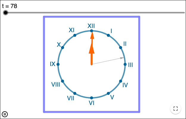
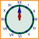
You can use a slider to export an animated gif. The animation must only rely on one slider, so if your animation uses several sliders, you must rewrite the slider dependencies using linearity. If you for instance want to use the resulting gif on a web page, don't use too many steps. Each step results in one image stored within the gif-file. The small gif to the right uses 140 steps and is 889 KB. The worksheet clock at the top of the page uses 43 200 steps and is saved in a file that is 18 KB (and the animation takes approximately 12 hours).
 '
'
How to make an animated clock
The video shows how to make an animated clock and export it to a gif-file.
Sliders that only tick
The normal usage of a slider is that some object uses the value of the slider for some purpose. You can also use sliders to make things happen. In the demonstration of Kepler's first law below, the value of the slider \(tick\) isn't used. It only ticks. The slider \(\alpha\) has the animation speed \(\alpha'\), whose value is given by
\[ \alpha'=speed\cdot \frac{\sqrt{a(1+e^2)}}{R^2} \]where \(e\) is the eccentricity and \(R\), as in a circular argument, depends on \(\alpha\),
\[ R = \frac{p}{1+e\cos(\alpha)} \]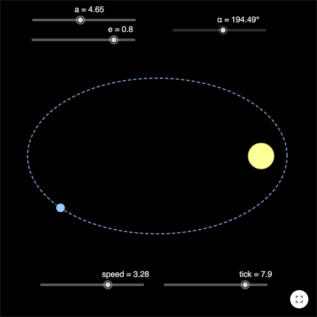
For details see the worksheet.
The Iteration command
With the command
Iteration( <Function>, <Start Value>, <Number of Iterations> )
you can apply a function on itself a number of times.
Let's say you want to show the trajectory of a cannon ball by repeatedly changing the velocity by the acceleration, and changing the position by the velocity. If the position is given by \((x,y)\), the velocity by \((vx,vy)\) and the acceleration by \((ax, ay)\), then the position will change as
\[ \begin{cases} x_{n} = x_{n-1}+vx \\ y_{n} = y_{n-1}+vy \end{cases} \]and the velocity as
\[ \begin{cases} vx_{n} = vx_{n-1}+ax \\ vy_{n} = vy_{n-1}+ay \end{cases} \]If modelling the gravity of the earth, the acceleration is constant.
By using an animated slider \(n\) in GeoGebra, a point \(Cannon\) and a point \(Ball\), you can let the point \(Ball\) get its value from
xpos = Iteration(x + vx, x(Cannon), n)
ypos = Iteration(x + vy, y(Cannon), n)
where the velocity gets its value from
vx = Iteration(x + xacc, vx0, n)
vy = Iteration(x + yacc, vy0, n)
where \(xacc, yacc, vx0\) and \(vy0\) get their values from sliders.
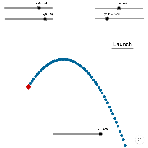
In the worksheet, the slider \(n\) has the animation property Increasing (Once) and the GeoGebra-script of the Launch-button is:
SetValue(n, 0)
StartAnimation(n)
by Malin Christersson under a Creative Commons Attribution-Noncommercial-Share Alike 2.5 Sweden License