Functions

There are a number of predefined functions and operators in GeoGebra that are shown on the site GeoGebra - Predefined Functions and Operators. In most cases it is easy to guess how a function should be written.

If you write an expression of \(x\) in the input bar, a function is created and given a name by GeoGebra. You can also name a function, for example by writing:

myFunction(x) = sin(x)

Using GeoGebra you can easily handle functions with coefficients. Let's say you want to show a polynomial function of degree three. You then make four sliders \(a, b, c, d\), and enter

f(x)=ax^3+bx^2+cx+d

in the input bar.

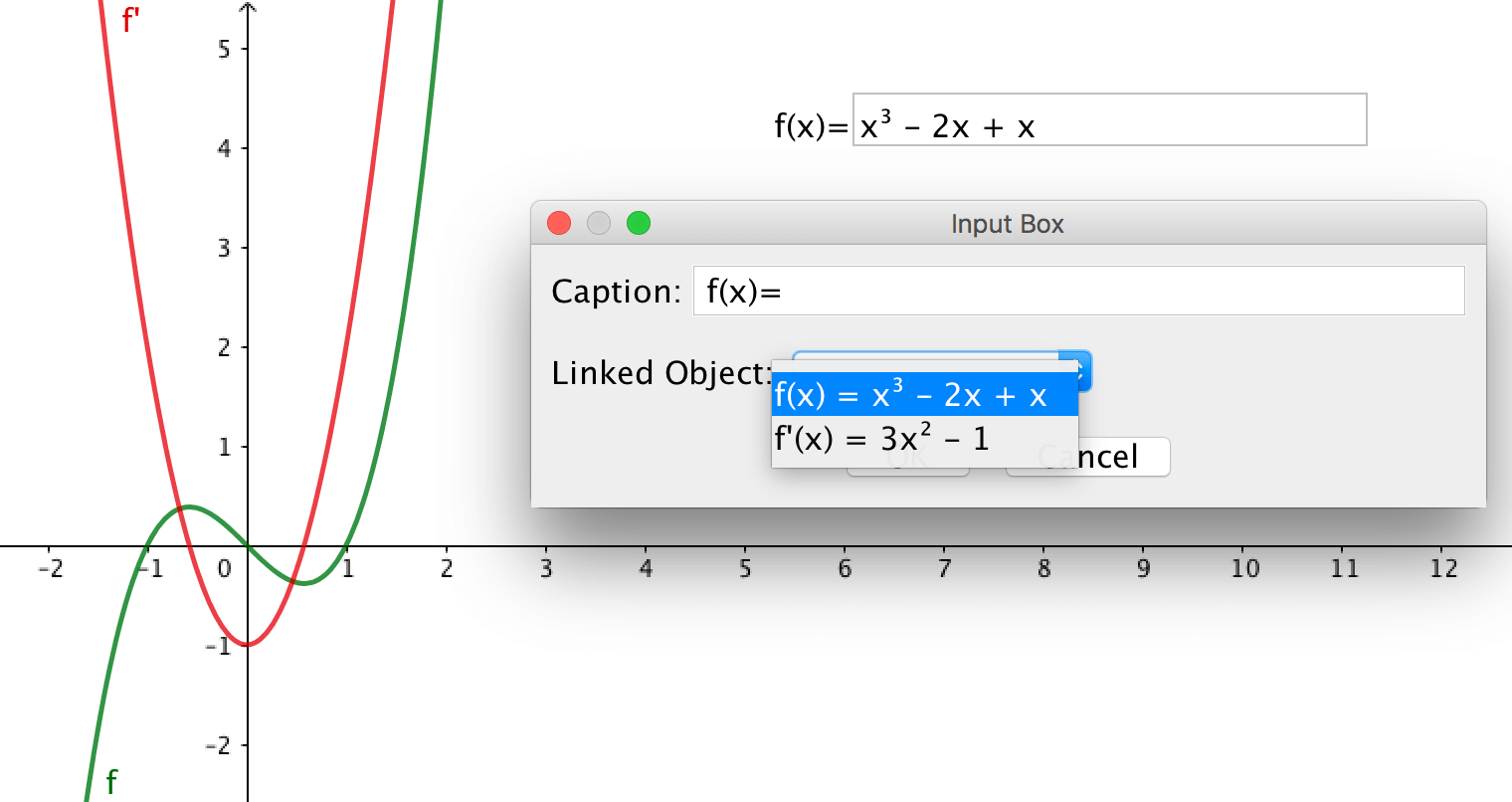
You can show a dynamic equation of the function by making a text object in the graphics view. Write f(x)= in the editing area and then choose \(f\) from the Object-menu.

The \(f(x)\)-notation and equations in \(y\) and \(x\)

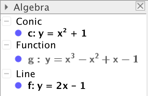
If you enter following functions in the input bar (one at a time):

y = 2x-1
y = x^2+1
y = x^3-x^2+x-1

and then look at the algebra view, you can see that GeoGebra treats them as three different kind of objects: a line, a conic section, and a function. All three objects are given names by GeoGebra.

A curve defined by an equation in \(y\) and \(x\) is a more general concept than a graph of a function. Not all such curves are graphs of functions.

As for lines, you can enter the equation x = 5 to get a vertical line, which isn't the graph of a function.

As for conic sections, you can enter the equation for any conic section. In the general case you can enter an equation

\[ax^2+bxy+cy^2+dx+ey +f=0\]

where the coefficients are either written as numbers or get their values from sliders.

The distinction made by GeoGebra (between lines, conic sections and functions) does not matter as long as you don't have to do any calculus. The commands used in calculus however, must work on objects that are functions. In that case, use \(f(x)\)-notation when entering the functions in the input bar, as in:

f(x) = 2x-1
g(x) = x^2+1
h(x) = x^3-x^2+x-1

Coefficients represented by sliders

For students starting to studying mathematical functions, denoting coefficients by letters, may be an abstraction that is difficult to grasp. In the expression

\[y = mx + c,\]

the letters \(y\) and \(x\) denote variables, whereas the letters \(m\) and \(c\) denote fix numbers. For absolute beginners, it may be a good idea to start by using examples where the coefficients are not represented by sliders.

\[ \begin{align*} y &= x \\ y &= -x \\ y &= 2x \\ y &= 2x +2 \\ y &= 2x -3 \end{align*} \]

When the students understand the concepts slope and \(y\)-intercept, you can introduce the sliders \(m\) and \(c\) to study a general linear function. Once the concept of coefficient is understood, sliders can be used for all functions.

Scale the axes

The easiest way to scale the axes is to hold down Shift and hover the mouse over one of the axes. When the cursor changes its appearance, you can drag that axis by holding down the left mouse button and drag.

You can also scale the axes by using the tool Move Graphics View and then drag the axes.

If you want to reset the ratio between the axes to 1:1, click Alt+M or Cmd+M. If you want another ratio, right click anywhere in the drawing pad where there is no object and choose xAxis:yAxis.

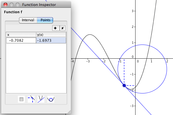
Function Inspector

Using the tool Function Inspector, you can inspect a function.

Using the function inspector, you can inspect a function in an interval

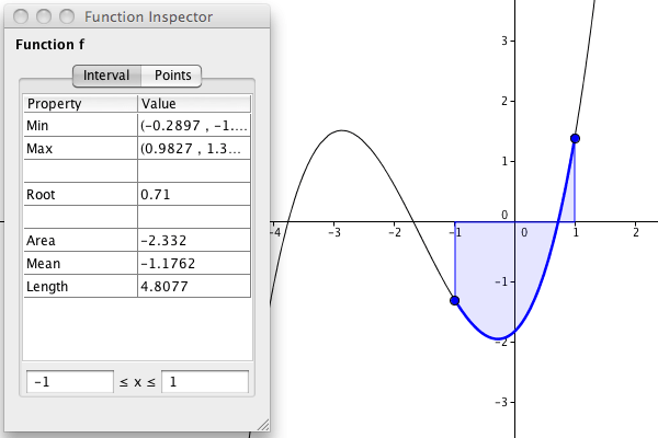
or around a point.

Degrees and radians

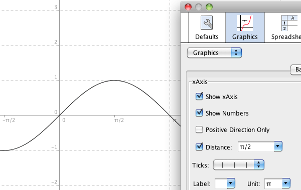
When you enter trigonometric functions, the default unit is radians. If you want to use radians, you can change the unit on the \(x\)-axis by right-clicking on the graphics view and pick Graphics.

If you want to use degrees, you have to add the degree-symbol when writing the function, as in: f(x)=sin(x° ). The short command for entering the degree-symbol is Ctrl+O.

Interactive Input Boxes

You can link an input box in the graphics view to a GeoGebra object. Use the tool Input Box and click in the graphics view. If you link an input box to a function, the equation of the function should be written using the same syntax as in the regular input box, for instance by using ^ for exponentiation.

Composite functions

If \(f\) and \(g\) are two functions that you have defined in GeoGebra, you can create a composite function by writing

f(g(x))

in the input bar.

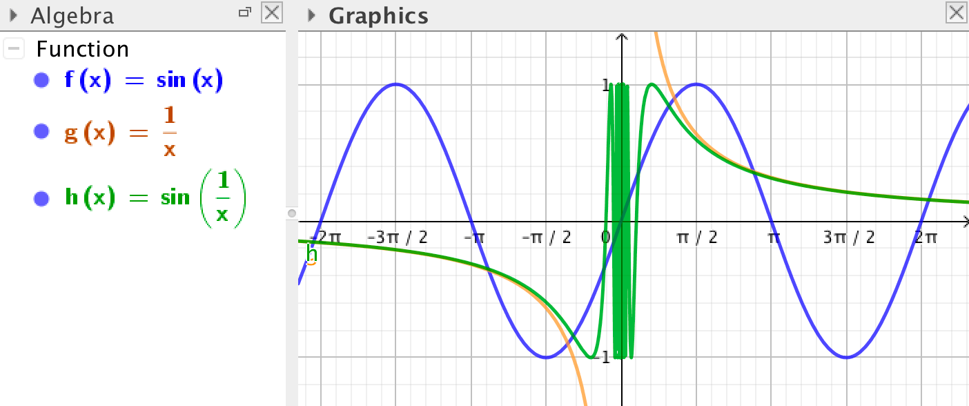
In the case where \(g(x) = \dfrac{1}{x}\) you can also enter

f(1/x)

or any other valid expression of \(x\) inside the brackets.

Inequalities

If you have two expressions in terms of \(x\), you can show for which intervals an inequality holds. As an example, you can enter following code in the input bar:

x^2<=x+1

This is how you write inequalities in GeoGebra: <, >, <=, >= stands for <, >, ≤ and ≥

Piecewise defined functions

A piecewise defined function is defined in different ways in different intervals. In GeoGebra you can define a function on an interval by using the command Function( <Function>, <Start x-Value>, <End x-Value> ).

The functions above are written:

f(x)=Function(1,-10,-1)
g(x)=Function(x^2,-1,1)
h(x)=Function(2x-1,1,10)
f_der(x)=Function(f'(x),-10,-1)
g_der(x)=Function(g'(x),-1,1)
h_der(x)=Function(h'(x),1,10)

Commands for functions

Given a function \(f\) you can write f'(x) in the input bar to create the derivative of the function.

By writing Integral( f, <Start x-Value>, <End x-Value> ) the integral is calculated and the area is shown in the graphics view.

If you place a point on the graph, the commands Curvature(<Point>, f) and CurvatureVector(<Point>, f) can be used to display the osculating circle.

If the function is a polynomial function you can also use the commands TurningPoint(f) and InflectionPoint(f).

You can use the command TaylorPolynomial(f, <x-Value>, <Order Number> ) to show the Taylor polynomial of a given order.

Riemann sums

There are predefined commands in GeoGebra to make Riemann sums. Given a function \(f\), you can make three different sorts of sums:

UpperSum(f, <Start x>, <End x>, <Number of Rectangles>)

LowerSum(f, <Start x>, <End x>, <Number of Rectangles>)

TrapezoidalSum(f, <Start x-Value>, <End x>, <Number of Trapezoids>)

Exercises

Exercise 1

Transformations of graphs

Part 1

Make a slider \(a\). Make a function \(f(x) = x^2\).

Make four functions \(g(x) = f(x+a)\), \(h(x) = f(x)+a\), \(p(x) = f(a\cdot x)\) and \(q(x) = a\cdot f(x)\).

Part 2

A worksheet with five functions may be hard to use due to the abundance of information it contains. You can use the tool Check Box to hide/show certain objects.

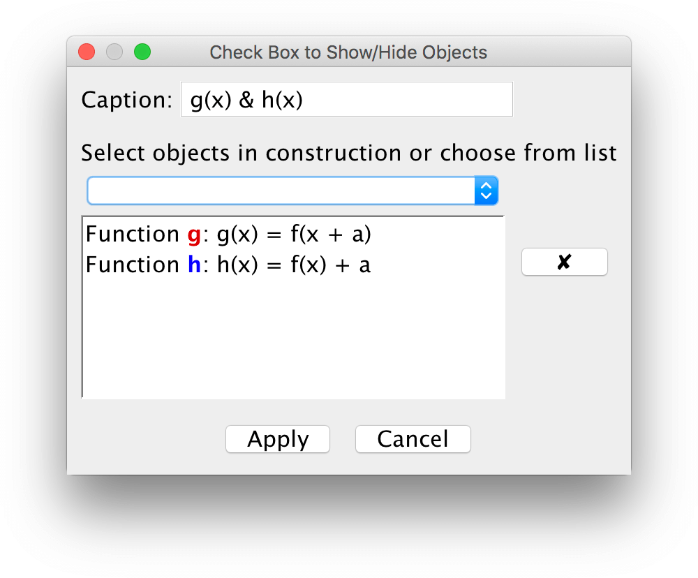
See to it that the functions \(g, h, p, q\) can be pairwise hidden/shown.

Since the conjectures you can make from studying transformations, hold for any function, it is good if the user can redefine the function \(f\). Use the tool Input Box to enable this.

If you also want informative text in the graphics view, add it!

Study how the graphs of the four functions change as you change the value of \(a\). Each transformation can be described either as a translation a certain amount of units in some direction, or as a shrink or stretch by some factor along som axis.

Describe each transformation. Specifically describe what happens when \(a = -1\). Some transformations are easier to see if \(f(x) = e^x\) or \(f(x) = \sin(x)\). Redefine \(f(x)\) using the input box.

Exercise 2

From unit circle to the sine function

Start by making sure that radians are used for measuring angles. Choose the menu Options -> Advanced and check Radians under the heading Angle Unit.

See to it that the \(x\)-axis has the distance \(\pi/2\).

Make a unit circle, three points, and an angle \(\alpha\), as in the figure below.

Create a point P = (α, y(A)) and drag the point \(A\) around the circle.

To clearly show that we are dealing with the \(y\)-coordinate, you can add two segments: Segment((x(A), 0), A) and Segment((x(P), 0), P).

Now there are various ways of showing the graph of the sine function. Try out all three!

Put a trace on the point \(P\) and drag the point \(A\).
Use the tool Locus. First click on \(P\) and then on \(A\).
Create a function with a restricted domain using the command Function( sin(x), 0, α ).

Exercise 3

From unit circle to the tangent function

Make a unit circle, three points, and an angle \(\alpha\). Also create the line \(x=1\).

Place a point \(B\) on the line \(x=1\) such that \(B\) also lies on the line between \(O\) and \(A\), as in the figure below.

Create a point \(P\) having the angle \(\alpha\) as \(x\)-coordinate and the same \(y\)-coordinate as the point \(B\).

Show the graph by: using a trace on \(P\), using the tool Locus, or by creating a function with a restricted domain. As in Exercise 2.

Exercise 4

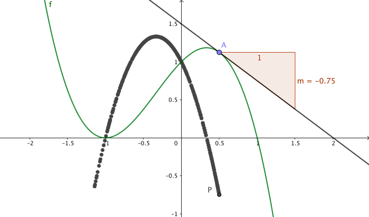
From slope to derivative

Define a function \(f(x) \) of your own choice. Place a point \(A\) on the graph. Use the tool Tangents to create a tangent to \(f\) through \(A\). Use the tool Slope to measure the slope of the tangent. The value of the slope is stored in a variable \(m\).

Create a point \(P\) having the same \(x\)-coordinate as \(A\) and the slope \(m\) as \(y\)-coordinate.

You can now show the graph of the derivative function in three ways.

Put a trace on the point \(P\) and drag the point \(A\).
Use the tool Locus. First click on \(P\) and then on \(A\).
Show the graph by writing f' in the input bar.

Exercise 5

From Riemann sums to integral

Input a function \(f\) of your own choice.
Insert a slider \(n\) of (positive) integer values. The slider represents the number of intervals.
Place two points \(A\) and \(B\) on the \(x\)-axis. The \(x\)-coordinates of the points are the end points of the interval.
Input the lower sum: L=LowerSum(f,x(A),x(B),n).
Input the upper sum: U=UpperSum(f,x(A),x(B),n).
Input the trapezium sum: T=TrapezoidalSum(f,x(A),x(B),n).
Input the integral: I=Integral(f,x(A),x(B)).