Vectors and Matrices
The movements of the ants are made using vectors.
Vectors
Vectors have a length and a direction. In GeoGebra you enter a vector either by using the tool ![]() or by writing a command the input bar.
or by writing a command the input bar.
See GeoGebra Tutorial - Points and Vectors for information about how GeoGebra treats points and vectors respectively. Vectors are often used to translate object.
Unit vectors
Unit vectors are vectors that have the length one unit. In GeoGebra you make a unit vector by using the command
UnitVector[< vector > ]
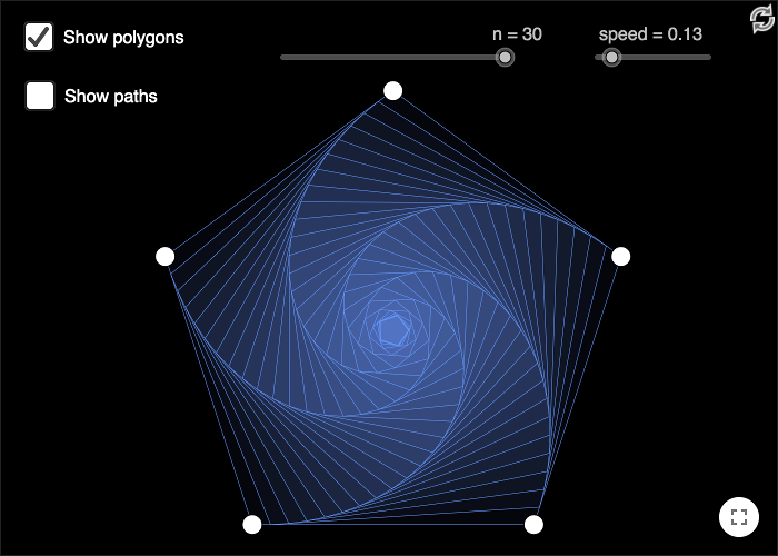
In the topmost worksheet, each ant moves in the direction to the next ant, in a clockwise order, and the length of the movement is given by the slider \(speed\). If \(A1\) and \(B1\) represent the positions of the first and second ants, then the next position \(A2\) of the first ant will be given by:
A2 = A1+speed*UnitVector[Vector[A1,B1]]
The easiest way to make a curve of pursuit in GeoGebra is to use the spreadsheet.
Translations along Two Vectors
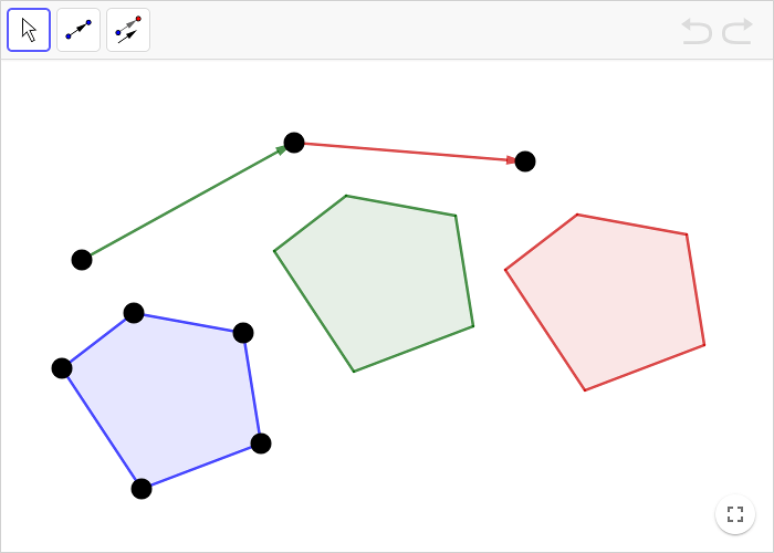
The blue polygon is translated along the green vector; the result is the green polygon. Then the green polygon is translated along the red vector; the result is the red polygon.
Make a new vector in the applet above.
Translate the blue polygon along your new vector.
How should you create your vector in order for the translated polygon to always overlap the red polygon?
If you succeed with the task, you have created a translation that has the same effect as two translations. This gives us a reasonable way of defining vector addition.
Adding Vectors
Vector addition is defined in the following way:
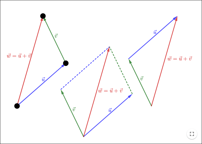
From the construction above you can see that \(\vec{w}=\vec{u}+\vec{v}=\vec{v}+\vec{u}\); changing the order of the vectors does not change the result, another word for this is that vector addition is commutative.
You can also represent vector addition graphically as a parallelogram.
Basis and Coordinates
A scalar is a real number. When doing vectors, you want to distinguish between quantities having a direction and quantities with no direction.
Task - Multiplication with a Scalar
Make a vector \(\vec{u}\) with its initial point at the origin.
Input
2*uin the input bar.Input
-uin the input bar.Change the vector
u.Make a slider \(a\). Input
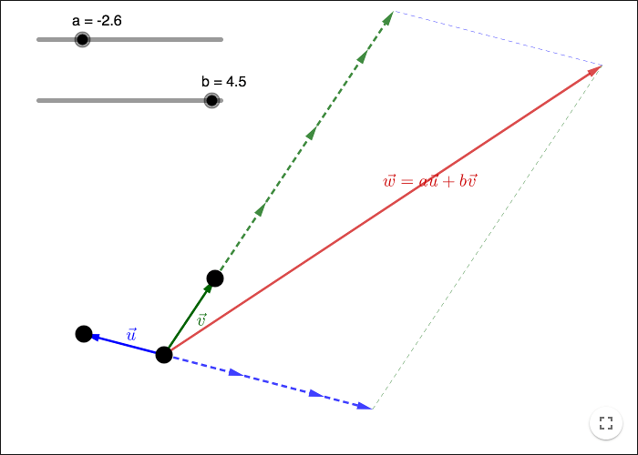
a*uin the input bar. Describe the result when multiplying a vector with a scalar; a positive or negative scalar.
What happens when multiplying with zero? Is the result still a vector? Would it be reasonable to define the "zero vector" as a vector or not? If it is a vector how does it differ from other vectors?
Some definitions
Any two non-zero vectors that are not parallel, form a basis for the plane. Given a basis you can describe any vector in the plane as a linear combination of the basis vectors.
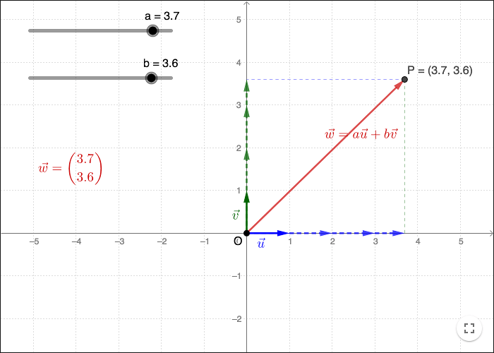
If the basis vectors are called \(\vec{u}\) and \(\vec{v}\), then any vector \(\vec{w}\) can be written as
\[\vec{w}=a\vec{u}+b\vec{v}\]
for some scalars \(a\) and \(b\). \(\vec{w}\) is a so called linear combination of \(\vec{u}\) and \(\vec{v}\). The scalars \(a\) and \(b\) are called the coordinates of \(\vec{w}\) in the basis \(\vec{u}\) and \(\vec{v}\).
If the basis is known, you can use a short form for writing the vector, either as
\[\vec{w}=(a,b) \hspace{1cm} \text{or} \hspace{1cm} \vec{w}=\binom{a}{b}\]
If you have two vectors \(\vec{w}=a\vec{u}+b\vec{v}\) and \(\vec{z}=c\vec{u}+d\vec{v}\), you can add them like this
\[\binom{a}{b}+\binom{c}{d}=a\vec{u}+b\vec{v}+c\vec{u}+d\vec{v}=(a+c)\vec{u}+(b+d)\vec{v}=\binom{a+c}{b+d}\]
In GeoGebra the Cartesian coordinate-system is used to define the basis vectors. The first basis vector is a vector from the origin to the point (1,0), the second vector is from the origin to the point (0,1). A basis for which each basis vector is a unit-vector, and where the basis vectors are mutually ortoghonal (perpendicular to each other), is called an orthonormal basis.
Bound Vectors
In a Cartesian plane, you can place a vector between points in the plane. By choosing the base vectors to have the initial points at the origin and their terminal points at (1, 0) and (0, 1) respectively, you get a convenient basis for comparing the coordinates of vectors and the coordinates of points.
The vector coordinates of \(\vec{w}\) are the same as the Cartesian coordinates of the terminal point \(P\) of \(\vec{w}\). You can describe the vector \(\vec{w}\) as the vector with the initial point \(O\) and the terminal point \(P\), where \(O\) is at the origin.
\[\vec{w}=\vec{OP}\]
\(\vec{OP}\) is a bound vector, it is a vector between the points \(O\) and \(P\) and as such it cannot be moved. If you want a movable vector, you introduce a vector \(\vec{w}\) and let \(\vec{w}=\vec{OP}\).
By applying vector addition repeatedly you find that \(\vec{z}=\vec{u}+\vec{v}+\vec{w}\); or in bound vectors
\[\vec{OC}=\vec{OA}+\vec{AB}+\vec{BC}\]
Subtracting vectors
When subtracting two vectors \(\vec{u}\) and \(\vec{v}\), you get the resulting vector, \(\vec{u}-\vec{v}\), by starting at the terminal point of \(\vec{v}\) and ending at the terminal point of \(\vec{u}\); as seen from the parallelogram in the construction below.
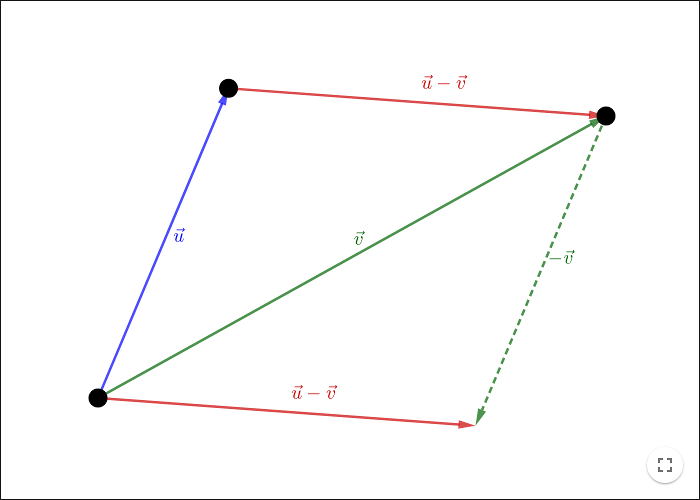
This result is especially important when trying to find the coordinates of bound vectors between points in the Cartesian plane.
If you have the vector \(\vec{PQ}\) between two points \(P\) and \(Q\) with known coordinates; you can find the coordinates of \(\vec{PQ}\) by using vector subtraction.
Since \(\vec{OP}\) and \(\vec{OQ}\) have the same coordinates as the points \(P\) and \(Q\), you can find the coordinates of \(\vec{PQ}\) by using the identity:
\[\vec{PQ}=\vec{OQ}-\vec{OP}\]
Equation of a line
You can write the equation of a line in parametric form using vectors.
Let \(l\) be line through a point \(A\) along a vector \(\vec{u}\). For any point \(P\) on the line, the equation
\[\vec{OP} = \vec{OA}+t\vec{u}\]holds for some \(t \in \mathbb{R}\).
Let \(\vec{r_0}= \vec{OA}\) and \(\vec{r}= \vec{OP}\), the equation of the line can be written using vectors as
\[\vec{r} = \vec{r_0}+t\vec{u}.\]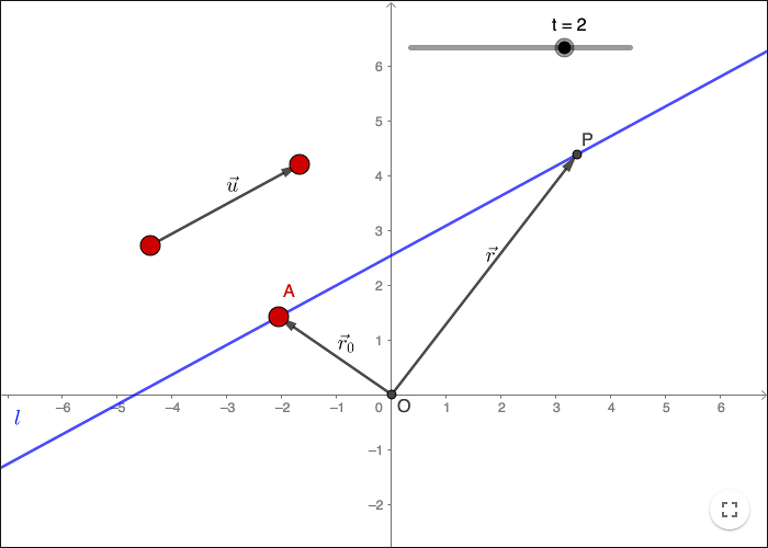
Matrices
The easiest way to create a matrix in GeoGebra is to use the spreadsheet. The matrix
\[\mathbf{A}=\left( \begin{array}{ccc} 1 & 2 & 3 \\ 4 & 5 & 6 \\ \end{array} \right)\]
is entered as in the picture below. Then you select the six cells and choose the spreadsheet tool "Create Matrix".
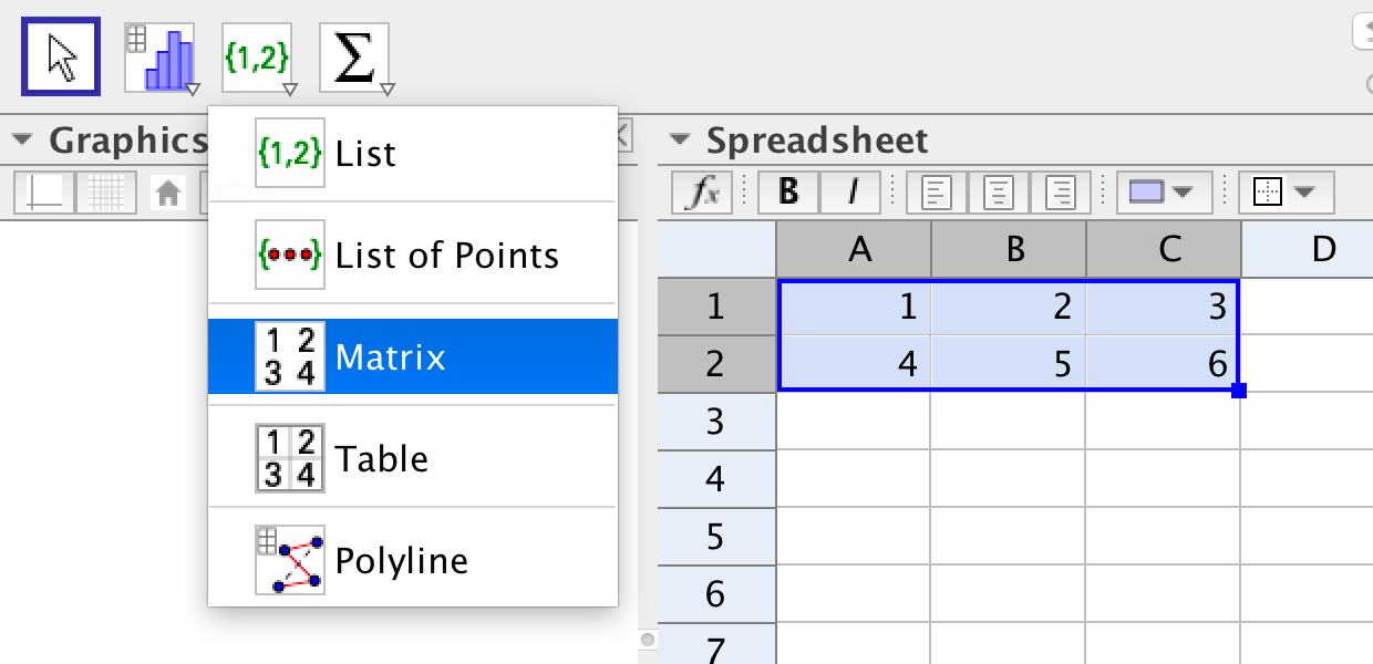
In the window that pops up, you can give the matrix a name before clicking on Create.
If you click on the small arrow below the input bar, you can find all commands for vectors and matrices.
As an example, you can create another matrix that is the transpose of \(\mathbf{A}\) by using the command
Transpose[A]
The transpose \(\mathbf{A^T}\) of a matrix \(\mathbf{A}\), is the result when swapping the columns and the rows.
\[\mathbf{A^T}=\left( \begin{array}{ccc} 1 & 4 \\ 2 & 5 \\ 3 & 6 \\ \end{array} \right)\]
If you want to use an element of a matrix, you can use the command
Element[<matrix>, <row>, <column>]
If you enter Element[A,2,3], 6 is returned.
Points/vectors and matrices in GeoGebra
A vector can be seen as a matrix with one column, a \(m\times 1\) matrix. The vector \(\mathbf{u}\) below is a \(2\times 1\) matrix.
\[\mathbf{u}=\left( \begin{array}{ccc} a \\ b \\ \end{array} \right)\]
Even though points and vectors/matrices are represented in different ways, you can multiply a matrix with a point.
Linear transformations
If the unit vectors \(\mathbf{e_1}\) and \(\mathbf{e_2}\) are mapped onto the vectors \(\mathbf{u}=\binom{a}{b}\) and \(\mathbf{v}=\binom{c}{d}\), then the transformation matrix is given by
\[\mathbf{T}=\left( \begin{array}{} a & c \\ b & d \\ \end{array} \right)\]
The absolute value of the determinant gives the scale factor of the areas. Check out the transformed image of the Mandelbrot set when the determinant is negative!
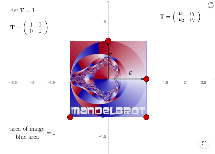
In order to visualize a linear transformation of a polygon in GeoGebra, do this:
Make two vectors \(\mathbf{u}\) and \(\mathbf{v}\) starting at the origin. Do not place the end points on the \(x\)- or \(y\)-axes or they will get stuck there. Rename the end point of \(\mathbf{u}\) to \(A\), and the end point of \(\mathbf{v}\) to \(B\).
Create the transformation matrix \(\mathbf{T}=\left( \begin{array}{} x(A) & x(B) \\ y(A) & y(B) \\ \end{array} \right)\)
Store the determinant in a variable:
detT=determinant(T)Make a polygon, \(poly1\).
Transform the polygon by using the command
ApplyMatrix[T,poly1]Make a variable:
areas=poly1'/poly1.Right click on \(poly1'\), choose Properties and then the Advanced tab. Input
detT>0in the field ”Blue”, anddetT<=0in the field ”Red”. The polygon will become red whenever the determinant is negative.Observe the variables \(areas\), \(detT\) and the colors of the polygon!
Linear transformations of curves
The blue graph, in the worksheet below, is transformed to the green graph by the matrix \(\mathbf{T}\).
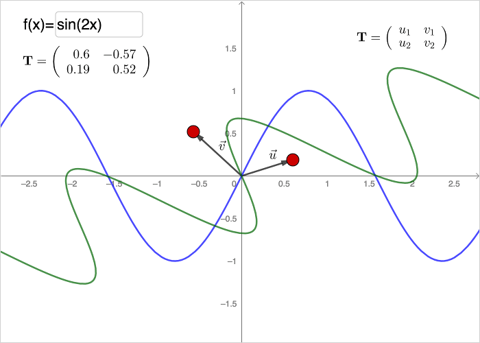
The graph of a function \(f(x)\) can be drawn as a curve \(c\) by writing the code:
c=Curve[t, f(t), t, -20, 20]
Each point on the curve has coordinates \((t,f(t))\). Applying a transformation matrix on the corresponding vector will yield the
transformed curve. To do it in GeoGebra, create points and vectors as described in the section above. Then use the command ApplyMatrix on the curve.
by Malin Christersson under a Creative Commons Attribution-Noncommercial-Share Alike 2.5 Sweden License