Fixpoints and Cobweb Plots
A recursive equation can be described in a general way like this
\[ \left\{ \begin{align*} a_0 &= c \\ a_{n+1} &= f(a_n),n\geq0 \end{align*} \right. \]
If \(a_n\) has a limit as \(n\rightarrow \infty\) , applying the function \(f\) on this limit will yield the same number again. The limit is called a fixpoint. If we call the limit \(x_0\), then
\[f(x_0)=x_0\].
You find the fixpoints to a recursive equation by solving the equation \(f(x)=x\).
When iterating the recursive equation, you apply the same function on itself over and over again.
\[x,f(x),f(f(x)),f(f(f(x))),\ldots \]
If the recursive equation is
\[ \left\{ \begin{align*} a_0 &= c \\ a_{n+1} &= 1+\frac{1}{a_n},n\geq0 \end{align*} \right. \]
the function of a function of a ..., becomes a continued fraction
\[1+\cfrac{1}{1+\cfrac{1}{1+\cfrac{1}{1+\cdots}}}\]If the recursive equation is
\[ \left\{ \begin{align*} a_0 &= c \\ a_{n+1} &= \sqrt{1+a_n},n\geq0 \end{align*} \right. \]the function of a function of a ..., becomes a continued square root
\[\sqrt{1+\sqrt{1+\sqrt{1+\sqrt{1+\cdots}}}}\]Attracting or repelling fixpoints
A fixpoint can be attracting or repelling.
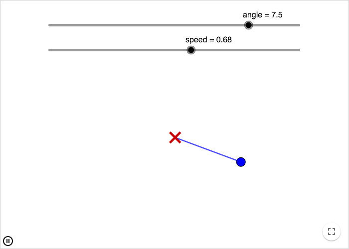
Damped pendulum
A damped pendulum has two fixpoints. One is when the pendulum is pointing down, at the angle 0, and one is when the pendulum is pointing up, at the angle π. In theory (not considering the Heisenberg uncertainty principle) if the pendulum starts at exactly the angle π it will stay there, this is a repelling fixpoint, but if you move it slightly it will eventually end up at the attracting fixpoint, the angle 0.
Repelling fixpoints
If the fixpoints are irrational numbers you will never find the repelling fixpoints when iterating a recursive equation. Even if you start at a repelling fixpoint, the iterations will result in values getting further and further away from the fixpoint. Regardless of how many correct decimals your electronic device can handle, it cannot handle infinitely many correct decimals; there will always be an error. In order to find the repelling fixpoints you need some other method.
For a recursive equation
\[ \left\{ \begin{align*} a_0 &= c \\ a_{n+1} &= f(a_n),n\geq0 \end{align*} \right. \]
solve the equation
\[f(x)=x\]
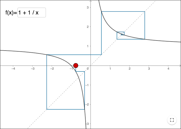
The fixpoints are the intersections between the line and the graph of the function.

You can use a picture like the one above to make a cobweb plot. Using a cobweb plot it is easy to see if a fixpoint is repelling or attracting.
Cobweb plots
Iterations of the recursive equation
\[ \left\{ \begin{align*} a_0 &= c \\ a_{n+1} &= 1+\frac{1}{a_n},n\geq0 \end{align*} \right. \]
can be illustrated by using a so-called cobweb plot.
Slope of the function
Any point that is "close enough" to an attracting fixpoint will end up at the fixpoint when iterated. The slope of the function at the fixpoint decides whether the fixpoint is repelling or attracting (or neither).
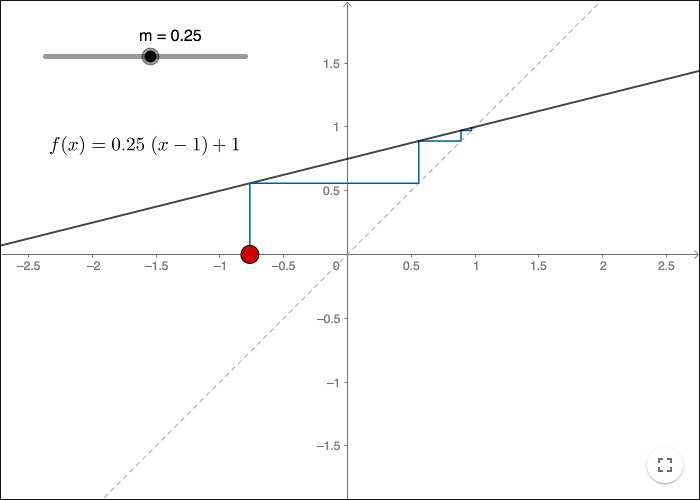
Find out for what slopes a fixpoint is attracting.
If you can classify a fixpoint of a linear function by the value of its slope, then you can classify a fixpoint for any other differentiable function by the value of the derivative at the fixpoint.
Exercises
Exercise 1
Find fixpoints
Find the fixpoints to the continued fraction
\[1+\cfrac{1}{1+\cfrac{1}{1+\cfrac{1}{1+\cdots}}}\]Find the fixpoints to the continued square root
\[\sqrt{1+\sqrt{1+\sqrt{1+\sqrt{1+\cdots}}}}\]
Exercise 2
Make a cobweb diagram using GeoGebra
- Input a function \(f(x) = 1+1/x\), a line \(y = x\) and a point \(A\) on the \(x\)-axis.
- Use the tool
 Perpendicular line and intersection points to mark all points of the diagram. Zoom in when you get close to the fixpoint.
Let the diagram start at the point \(A\).
Perpendicular line and intersection points to mark all points of the diagram. Zoom in when you get close to the fixpoint.
Let the diagram start at the point \(A\). - Hide all lines and create segments between the points. Hide all points except for \(A\).
- Choose the tool
 Input box and link it to the function \(f(x)\).
Exercise 3
Make a cobweb diagram using the spreadsheet.
- Input a function \(f(x) = 1+1/x\), a line \(y = x\) and a point \(A\) on the \(x\)-axis.
- Choose
View -> Spreadsheetin the menu.- Enter
x(A)in cell A1. - Enter
f(A1)in cell B1. - Enter
(A1, B1)in cell C1. - Enter
(B1, B1)in cell D1. - Enter
x(D1)in cell A2.
- Enter
- To show the segments:
- Enter
Segment(C1, D1)in cell E1 - Enter
Segment(C2, D1)in cell F2
- Enter
- Make relative copies.
- Choose the tool Input box and link it to the function \(f(x)\).
Exercise 4
Repelling and attracting fixpoints
Use a GeoGebra-file showing a cobweb diagram. Create a slider m and check out the diagram using the function:
\[f(x) = 1+m x\]For what slopes is the fixpoint attracting/repelling?
Exercise 5
Logistic map
Use a GeoGebra-file showing a cobweb diagram. Create a slider r and check out the diagram using the function
\[f(x) = r x\cdot (1-x)\]where \(0\le r \le 4\). Try to find values of r that illustrate:
- convergence towards \(0\).
- convergence towards a fixpoint \(\ne 0\).
- jumps between two values.
- jumps between four values.
- a seemingly chaotic behavior.
by Malin Christersson under a Creative Commons Attribution-Noncommercial-Share Alike 2.5 Sweden License