Integrals
One way to approximate the area under a graph is to approximate the area by using a number of rectangles. A number of rectangles approximating the area under a graph is called a Riemann sum.
When making the rectangles, there are two standard ways if doing it. In GeoGebra you can use two commands, let \(f\) be the function, \(a\) the first \(x\)- value and \(b\) the second, and let \(n\) be the number of rectangles, then you can write
UpperSum( f , a, b, n )
or
LowerSum( f , a, b, n )
The function must be defined on the interval \([a, b]\).
You can see the difference between the two commands in the worksheet below.
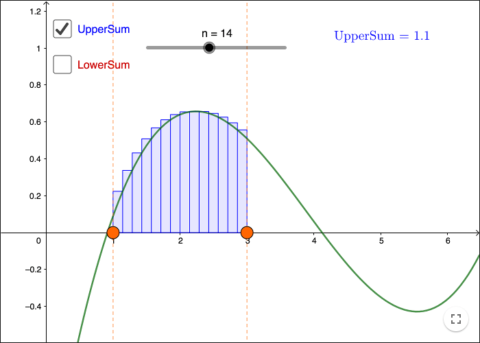
Note that if you try to approximate the area between \(x = 5\) and \(x = 6\), you get a negative value. Since an area cannot be negative, it's not really the area you get from Riemann sums. You either get the area or the negative value of the area, depending on whether the graph is above or below the \(x\)-axis.
To handle area under graphs algebraically, you use so called integrals. Integrals can be defined using Riemann sums, as the limit when the number of rectangles tend to infinity.
So why would anyone be interested in finding the area under a graph. One concrete example has to do with distance and speed. If you know the speed of an object, you can find the distance travelled by calculating ‐ the area under a graph.
Distance and speed
If an object moves at a constant speed during a time interval \(\Delta t\), then following relations are true for the distance, \(\Delta s\), and the speed \(v\):
\[v=\frac{\Delta s}{\Delta t} \hspace{0.5 cm} \text{and} \hspace{0.5 cm} \Delta s = v\cdot \Delta t\]Graphically, you get the speed by taking the slope of the segment representing the function \(s(t)\). You can get the total distance traveled either by using the function \(s(t)\) or the constant function \(v(t)\).


If the function \(s(t) \) isn't a linear function, if the speed isn't constant, then you can approximate \(s(t)\) with a function that is linear within time-steps, and then use the same line of reasoning. The smaller time-steps you use, the better approximation you get.
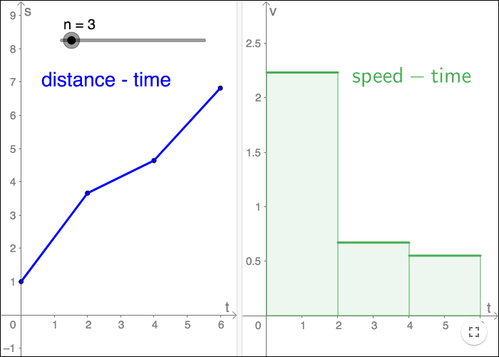
If you divide the time into intervals, where you have a constant speed within each interval; then you get the speed within an interval by taking the slope of the segment belonging to that interval in the distance-time diagram.
To find the total distance traveled, you can add the areas of the rectangles, this will yield an approximation of the total distance travel.


If you let the number of intervals tend to infinity, then \(\Delta t \rightarrow 0\). You can now find the speed at a given point by differentiating at that point.
\[v=\frac{ds}{dt}\]
As \(\Delta t \rightarrow 0\), the area under the graph of \(v(t)\) tends to the total distance travel, i.e. \(s(b)-s(a)\).
If we know the function \(v(t)\), but not the function \(s(t)\), then we can find the area under the graph by first finding a function whose derivative is \(v(t)\). We do the opposite of finding the derivative.
Antiderivative
The antiderivative, or primitive function, of a function \(f(x)\), is a function \(F(x)\) such that \(F'(x) = f(x)\).
A function \(f\) has infinitely many different antiderivatives. The functions
\[ \begin{align} F_1(x) &= \frac{x^2}{2}+5 \\ F_2(x) &= \frac{x^2}{2} \\ F_3(x) &= \frac{x^2}{2}-300 \end{align} \]are all antiderivatives to the function \(f(x)=x\).
When finding the antiderivative to a function, you usually add a constant \(C\), to get all antiderivatives. The function
\[F(x) = \frac{x^2}{2}+C, \]where \(C\) is a constant, is the antiderivative to \(f(x) = x\).
From Riemann sum to integral

The area of the step function in the picture above is
\[A=f(x_0)\cdot \Delta x + f(x_1)\cdot \Delta x + f(x_2)\cdot \Delta x + f(x_3)\cdot \Delta x + f(x_4)\cdot \Delta x \]Let \(F(x)\) be an antiderivative to \(f(x)\), i.e. a function such that \(F'(x)=f(x)\). If \(\Delta x\) is "small", we can make following approximation
\[f(x_i)\approx \frac{F(x_{i+1})-F(x_i)}{\Delta x} \text{ for } i=0,1,2,3,4\]This gives us following approximation for the area
\[A\approx \frac{F(x_1)-F(x_0)}{\Delta x}\cdot \Delta x + \frac{F(x_2)-F(x_1)}{\Delta x}\cdot \Delta x + \frac{F(x_3)-F(x_2)}{\Delta x}\cdot \Delta x \\ + \frac{F(x_4)-F(x_3)}{\Delta x}\cdot \Delta x + \frac{F(x_5)-F(x_4)}{\Delta x}\cdot \Delta x \]Cancel out all \(\Delta x\)
\[ \begin{align} A &\approx F(x_1)-F(x_0) + F(x_2)-F(x_1) + F(x_3)-F(x_2) + F(x_4)-F(x_3) + F(x_5)-F(x_4)\\ &=F(x_5)-F(x_0) \end{align} \]Let the number of intervals tend to infinity, then \(\Delta x \rightarrow 0\). If the endpoints are called \(a\) and \(b\), we get that
\[A=F(b)-F(a)\]
The area \(A\) is a limit of a sum of terms of the form
\[f(x_i)\Delta x.\]We write \(A\) using an integral-symbol, which looks like an S-shaped version of the sigma-symbol ( \(\sum\) ) used for sum. The endpoints of the interval is written below and above the integral-symbol.
\[A = \int_a^b\! f(x) \,dx \]Sometimes the integral-symbol without any endpoints of an interval, is used to denote the antiderivative.
\[\int\! f(x) \,dx = F(x) \]Fundamental theorem of calculus
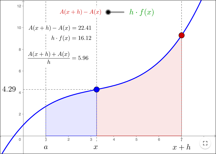
Let \(f(x)\) be a continuous function on an interval \([a, b]\). We can define a function \(A(x)\) as the area under the graph of \(f(x)\) on the interval \([a,x]\).
According to the fundamental theorem of calculus,
\[A'(x) = f(x)\]for all \(x\in [a, b] \).
In order to show this theorem, we must show that
\[\lim_{h\rightarrow 0}\frac{A(x+h)-A(x)}{h}=f(x)\]The line of reasoning is sketched out in the worksheet below.
Since all antiderivative functions to a given function just differ by a constant, you can use any such function when calculating the area under \(f(x)\) in the interval \([a,b]\). Let \(F(x)\) be an antiderivative to \(f(x)\), then \(F(x)=A(x)+C\) for some constant C. Then
\[\int_a^b \! f(x) \, dx = F(b)-F(a)=A(b)+C-(A(a)+C)=A(b)-A(a)=A(b)-0=A(b)\]Hence, if \(F(x)\) is any antiderivative function to \(f(x)\), then
\[ \frac{d}{dx} \int_a^x\! F(x)\, dx = f(x).\]by Malin Christersson under a Creative Commons Attribution-Noncommercial-Share Alike 2.5 Sweden License