Normal Distribution
From discrete to continuous
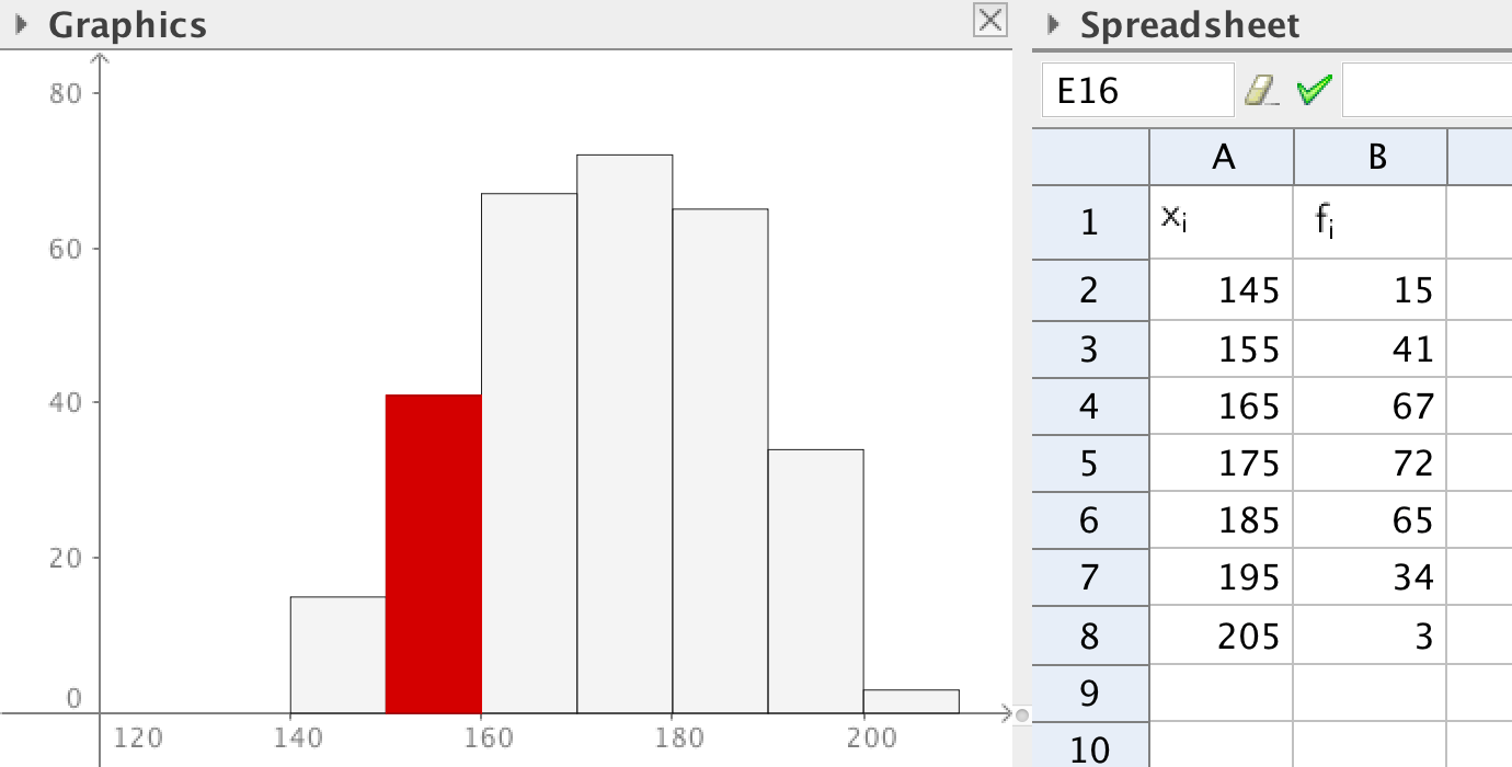
The probability that a person picked at random has a height between 150 and 160 cm can be calculated from the table:
\[p=\frac{41}{15+41+67+72+65+34+3}\]
You could also find the probability by looking at the areas of the bars in bar chart. The probability is then found by dividing the area of the red bar by the total area.
\[p=\frac{41\cdot 10}{15\cdot 10+41\cdot 10+67\cdot 10+72\cdot 10+65\cdot 10+34\cdot 10+3\cdot 10}\]
Probability and area
One way of illustrating the probability that an outcome is in a certain interval, is to let the area of the interval be the probability. The total area must in this case be one. A new bar chart having the same appearance but the total area of one can be constructed.
Exercise 1
Add another column in the spreadsheet representing the relative frequency.
You can add a number of values in cells by writing:
Sum(B2:B8)
If you make a bar chart using the relative frequency instead of the absolute frequency, the total area will still not be one. Add another column where you normalize the relative frequencies in order to get the total area one. How do you construct this column? The column for the data should not be changed. Draw the bar chart!

Exercise 2
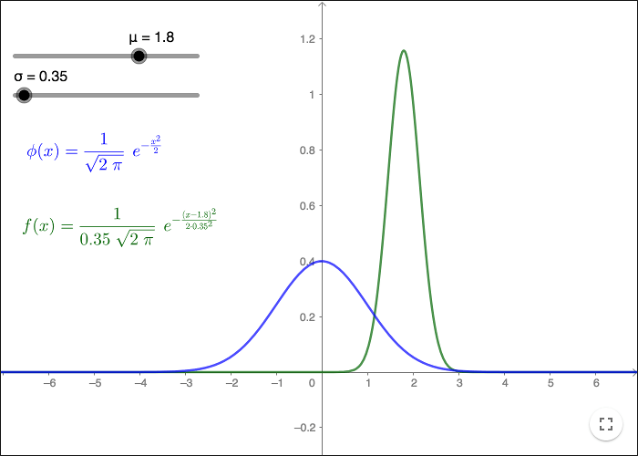
You can approximate a discrete distribution of data values with a continuous function. One such approximating function is the normal probability distribution function (normal pdf). The graph of the normal pdf is a completely symmetric bell-shaped curve whose appearance depends only on two values; the mean and the standard deviation.
If \(\mu\) is the mean value and \(\sigma\) the standard deviation, the normal pdf is:
\[f(x)=\frac{1}{\sigma \sqrt{2\pi}}e^{\left( - \dfrac{(x-\mu)^2}{2\sigma^2}\right)} \]
Use the mean 173.2492 and the standard deviation 14.0333 to plot the graph of the normal distribution.

Standard normal distribution
The pdf for the standard normal distribution \(\phi\), has mean \(\mu =0\) and standard deviation \(\sigma=1\).
\[\phi (x)=\frac{1}{\sqrt{2\pi }} e^{-\frac{1}{2}x^2} \]
A short form for writing that a random variable \(X\) is distributed normally with mean \(\mu\) and standard deviation \(\sigma\), is to write: \(X\ \sim \mathcal{N}(\mu,\sigma^2)\). A variable that is distributed by the standard normal distribution is denoted \(Z\). The correspondence between \(Z\) and \(X\) is
The probability is given by the area under the curve. The total area is therefore always one. If the random variable is denoted \(X\), then the probability \(P\) is given by
\[P(a\lt X \lt b)=\int_a^bf(x)dx\]
where \(f(x)\) is the normal pdf.
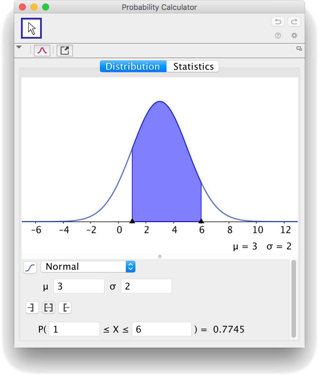
Normal distribution in GeoGebra
By using the tool
![]() Probability Calculator,
you can find the probability between boundaries for a number of distribution functions. The tool is found in the menu belonging to the spreadsheet.
Probability Calculator,
you can find the probability between boundaries for a number of distribution functions. The tool is found in the menu belonging to the spreadsheet.
The inverse normal problem
If you know the mean and the standard deviation, you can find the probability between given boundaries by using the "Probability Calculator".
The inverse problem is that you know the probability for given boundaries and want to find the mean and the standard deviation. Since there are two unknowns to be found, you must know two probabilities. The problem is solved by using the correspondence with the standard normal pdf.
Suppose that you know that \(P(X\lt 4)=0.4\) and \(P(X\lt 3)=0.2\). The boundaries 4 and 3, can be compared to the corresponding boundaries for the standard normal pdf. The correspondence between these boundaries is \(z=\frac{x-\mu}{\sigma}\), where \(z\) is the boundary for the standard normal pdf, and \(x\) is the boundary for the unknown normal pdf.
To find the boundaries corresponding to 4 and 3, you can use GeoGebra. You must find \(z_1\) from \(P(Z\lt z_1)=0.4\) and \(z_2\) from \(P(Z\lt z_2)=0.2\).
Input 0.4 in the box shown in the picture below and press Enter. You get \(z_1=-0.2533\).
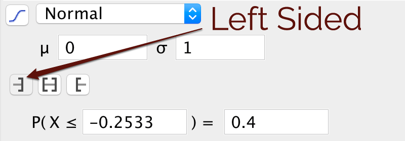
In a similar way you get \(z_2=-0.8416\). To find \(\mu\) and \(\sigma\), solve the simultaneous equations:
\[\left\{ \begin{align*} -0.2533&=&\frac{4-\mu}{\sigma} \\ -0.8416&=&\frac{3-\mu}{\sigma} \end{align*} \right. \]
A graphical solution is shown below.
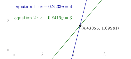
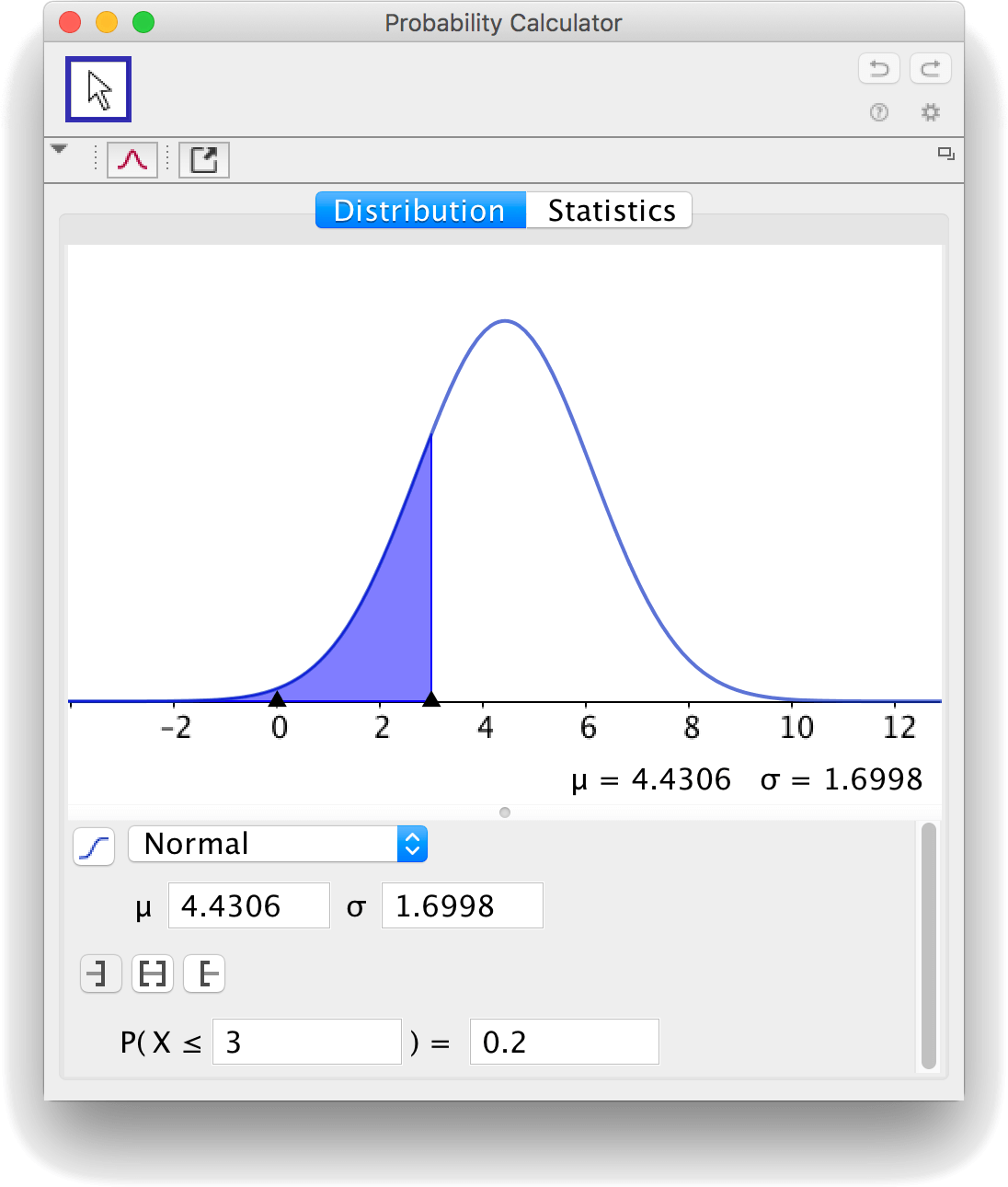
The solution is \(\mu=4.4306\) and \(\sigma=1.6998\). You can check the solution by using the "Probability Calculator".
by Malin Christersson under a Creative Commons Attribution-Noncommercial-Share Alike 2.5 Sweden License