Newton Fractals

Malin Christersson ◊◊◊ 2013-02-17

←Modelling 3D Illusions	Damped Lissajous Curves→

Treriksröset

There are infinitely many points on the borders between Finland, Sweden and Norway. All such points, except one, are points on the border between two countries. If you make a small circle around such a point, the circle will always overlap two different countries; no matter how small the circle is. One and only one point, is on the border of three countries. Any circle around this point, will always overlap three different countries. This point is called Treriksröset.

Each country on the map can be described as a set of points. A point that lies on the boundary to a set of points, is called a boundary point of the set. A boundary point does not belong to the set itself. Any circle around a boundary point of a set; will contain points both inside and outside of the set, no matter how small the circle is.

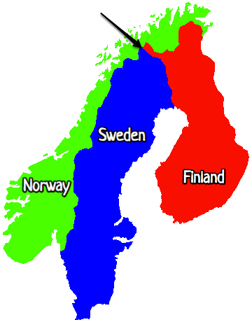
Now try to imagine three sets of points such that all boundary points are boundary points of all three sets! All boundary points should be like Treriksröset.

A Julia set

If three sets (coloured red, green, blue) must have no boundary between two colours only, then any area between two coloured regions must be filled with blobs of the third colour. A red region lying next to a green region, must be separated by a blue blob. The blue blob must have a small red blob separating it from the green region, and a small green blob separating it from the red region. This pattern must go on to infinity. An example of three such coloured sets, is shown below.

Three coloured sets. Click anywhere in the canvas to zoom in.

If all boundary points to three coloured sets, are boundary points to each of the three sets, then all three sets must have exactly the same boundary. This boundary is not visible in the canvas above but it is visualized in the canvas below. The boundary is an example of a so called Julia set.

The boundary is a Julia set. Click anywhere in the canvas to zoom in.

In the canvas below, the same set is shown using a different colouring scheme.

Click anywhere in the canvas to zoom in.

The three canvases above are created by iterating over points in the complex plane. The points are found by using the Newton-Raphson method to find an approximate solution to a polynomial equation. The fractals above are so called Newton fractals.

The Newton-Raphson method

The Newton Raphson method is used for approximating a root of an equation \(f(x)=0\). By starting at a point \((x_0, f(x_0))\) close to the root, it is possible to get a better approximation by following the tangent line to the \(x\)-axis. If the tangent intercepts the \(x\)-axis at a point \((x_1,0)\), the slope of the tangent is given by:

\[f'(x_0)=\frac{f(x_0)}{x_0-x_1}\]

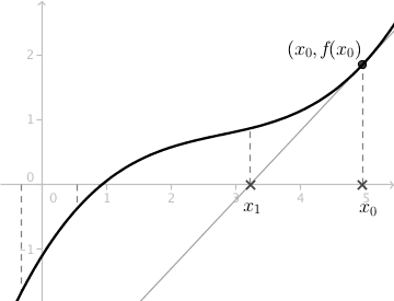
After rearrangement, the new approximation \(x_1\) is given by:

\[x_1=x_0-\frac{f(x_0)}{f'(x_0)}\]

The process can be repeated by using the same procedure on the new value \(x_1\). A general formula for finding a new approximation \(x_{n+1}\), given a value \(x_n\), is given by:

\[x_{n+1}=x_n-\frac{f(x_n)}{f'(x_n)}\]

Using GeoGebra, the spreadsheet can be used to find successive values of \(x_n\).

Enter a function \(f(x)\) and place a point A on the graph of the function. Let the \(x\)-value of A be the starting value \(x_0\).
Enter x(A) into cell A1 and enter A1-f(A1)/f'(A1) into cell A2.
Make relative copies along column A.

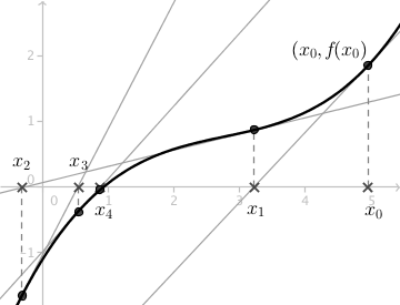
In order to demonstrate the process interactively; points, lines and segments can be created in the spreadsheet. A static example of the process is shown in the picture to the right.

By dragging the point A along the graph, and by varying the function, one can see that the points generated by the Newton-Raphson method converge rapidly to the intersection between the graph and the \(x\)-axis. For some initial values however, the method doesn't converge at all.

The Newton-Raphson method applied to complex functions

The Newton-Raphson method can be applied to complex functions as well.

Let the function be \(f(z)=z^3-1\). The equation \(f(z)=0\) has three roots: \[1, -\dfrac{1}{2}+\dfrac{\sqrt{3}}{2}i,-\dfrac{1}{2}-\dfrac{\sqrt{3}}{2}i \]

You don't need a computer to find the roots of the equation, but when the Newton-Raphson method is used to find approximate roots, a fractal pattern appears.

How to do it using GeoGebra

Using GeoGebra, it is just as easy to use the Newton-Raphson method on complex points, as it is to use it on real numbers.

Enter a complex number \(z_1\) into the graphics view.
Enter \(z_1\) into cell A1 and the code A1-(A1^3-1)/(3A1^2) into cell A2.
Make relative copies along column A.

When the complex number \(z_1\) is moved, one can clearly see that the iterated complex points converge to one of the three roots. In the demo below, there are vectors between successive points and all points have "Trace on".

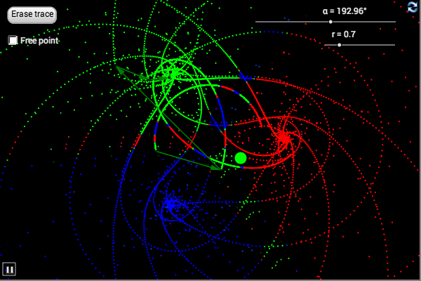
newton fractal — Move the point! Uncheck "Free point" to draw the circular path defined by the sliders.

The points can be coloured depending on which of the three roots they converge to. If A20 is the last cell used for the successive points, following code can be used for storing the colours in three variables.

red = If[abs(A20 - 1) < 0.1, 1, 0]
green = If[abs(A20 - (-0.5 + 0.866ί)) < 0.1, 1, 0]
blue = If[abs(A20 - (-0.5 - 0.866ί)) < 0.1, 1, 0]

The dynamic colours of the points can be specified under the Advanced tab in the Object properties window. Input the variables defined above in the colour fields. Note that a maximum colour value is given by 1, not by 255 which is the regular way to specify a rgb-value.

In order to make a finer picture, some programming language must be used.

Fixed points, basins of attraction, and Julia sets

A fixed point is a point that is mapped to itself under an iterated function. The three roots to the equation \(z^3=1\), are mapped to themselves under the iterative function \[z_{n+1}=z_n-\frac{z_n^3-1}{3z_n^2}\]

A fixed point is an attracting fixed point if all points in a neighbourhood around it converge towards it. All points that converge to a fixed point, form a basin of attraction for the point.

The Newton fractal has three basins of attraction; the red, green, and blue regions in the canvases above. The only points that do not converge to any of the three fixed points, are the points on the boundary of the basins of attraction. These boundary points form a Julia set. The boundary points have a chaotic behaviour.

The closer a point is to the boundary, the longer it will take to converge to one of the fixed points. It's this "distance" that is used to make the colouring of the black-and-white-canvas, and the multiple-colour-canvas above.

Julia sets are often shown as sets of points that fill up areas. These kind of Julia sets, are so called filled-in Julia sets. An interactive example of a filled-in Julia set is shown at malinc.se (the filled-in Julia sets are yellow). The true Julia set however, is only the boundary.