Damped Lissajous Curves

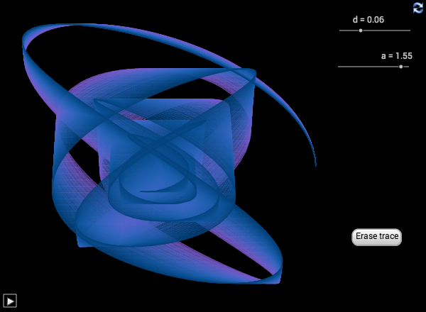
The curve is defined by the parametric equations:

\[\begin{cases} x(t) &= \cos(at)e^{-dt} \\ y(t) &= \sin(t)e^{-dt} \end{cases} , 0\leq t \lt 14\pi\]

The angular frequency of the \(x\)-coordinate, \(a\), varies between 0 and 2 as the curve is animated.

When \(d=0\), the curve is defined by:

\[\begin{cases} x(t) &= \cos(at) \\ y(t) &= \sin(t) \end{cases} , 0\leq t \lt 14\pi\]

This is a so called Lissajous curve (Wikipedia: Lissajous curve ). In this case, the \(x\)- and the \(y\)-coordinates are simple harmonic oscillators. When \(a=1\), the curve is a circle.

When \(d\gt0\), the amplitudes of the oscillations of the coordinates decay exponentially through the factor \(e^{-dt}\). In this case the coordinates are damped harmonic oscillators and the curve is a damped Lissajous curve. In this case, when \(a=1\), the curve is a spiral.

Harmonograph using GeoGebra

A harmonograph is a mechanical device that uses pendulums to control the movement of a pen and/or to control the movement of the drawing paper. When two pendulums that swing in perpendicular planes are used, the curve created will be a damped Lissajous curve. One such example, where the pendulums control the pen, is shown in this YouTube film. The curve created by a mechanical device, is usually longer than the curves shown above. Furthermore, the amplitude as well as the phase of the respective pendulum oscillation, may vary.

The behaviour of a harmonograph can be visualized using GeoGebra. Enter three sliders a, d, and t to represent the parameters of the curve traced out by the point:

\[( \cos(at)e^{-dt}, \sin(t)e^{-dt})\]

Let A and B be points representing the oscillating coordinates.

A=(cos(a t) e^(-d t), -1.5)
B=(-1.5, sin(t) e^(-d t))

Enter lines as in the worksheet below and enter the intersection point (the pen). Put a trace on the intersection point and animate t.

Load GeoGebra worksheet

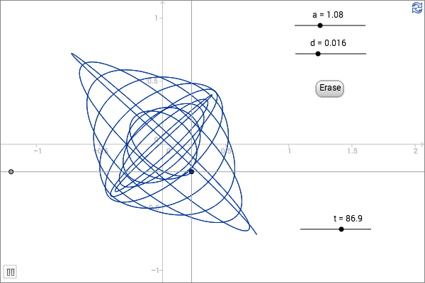
The curve traced out can be defined as a GeoGebra curve.

c=Curve[cos(a t) e^(-d t),sin(t) e^(-d t),t,0,6pi]

If animating the slider a, the colour of the curve can be specified as a function of a in the properties window under the advanced tab. In the example below, following functions for red, green and blue have been entered

(1 + cos(10a)) / 2.5
(1 + cos(13a)) / 5
(1 + sin(10a)) / 2.5

Load GeoGebra worksheet