2D & 3D Plots

2D Plots

Gnuplot on Mac

Octave uses gnuplot when plotting. If you use Mac, you must make sure gnuplot works. You might need to reinstall gnuplot with x11 support by using homebrew:

brew uninstall gnuplot;brew install gnuplot --with-x

Then start Octave and write:

setenv("GNUTERM","X11")

For troubleshooting check out this.

Plot using Octave

When plotting in Octave you plot points having their x-values stored in one vector and the y-values in another vector. The two vectors must be the same size.

You can use a x-vector to store the x-values; then you use element by element operations on the x-vector to store the function values in a y-vector. Having two vectors like this, you then use the command

plot(x_vector, y_vector)

>>> x=-2:2
x =

-2 -1 0 1 2

>>> y=x.^2
y =

4 1 0 1 4

>>> plot(x,y)

Octave inserts lines between the points. If you want a smoother graph, make a longer x-vector.

>>> x=-2:0.5:2;
>>> y=x.^2;
>>> plot(x,y)

If you know how many points you want to plot in an interval, you can let Octave space the points linearly by using the command

linspace(first x-value, last x-value, number of evenly spaced points)

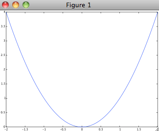
>>> x=linspace(-2, 2, 500);
>>> y=x.^2;
>>> plot(x,y)

3D - the grid

If we have a function of two variables \(z=f(x,y)\), we need three axes to display the graph.

When plotting in 2D we use evenly spaced x-values and function values of these stored in a y-vector.

When plotting in 3D we need evenly spaced x- and y-values, spaced on a grid where each function value z is taken of a point (x, y) on the grid. In order to achieve this we use the command meshgrid.

>>> x=linspace(-2,2,5)
x =

-2 -1 0 1 2

>>> y=linspace(-2,2,5)
y =

-2 -1 0 1 2

>>> [xx,yy]=meshgrid(x,y)
xx =

-2 -1 0 1 2
-2 -1 0 1 2
-2 -1 0 1 2
-2 -1 0 1 2
-2 -1 0 1 2

yy =

-2 -2 -2 -2 -2
-1 -1 -1 -1 -1
0 0 0 0 0
1 1 1 1 1
2 2 2 2 2

Each point on the grid is made by taken an element from the xx-matrix as the x-value and the corresponding element from the yy-matrix as the y-value. All in all there are 25 points in this grid.

Plot a 3D graph

After having made a grid you can plot a 3D graph using the command mesh(xx,yy,z), where xx and yy are the matrices made by meshgrid and where z is a function of x and y. You get the function values of z by using element by element operations on matrices xx and yy.

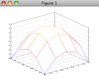
>>> x=linspace(-2,2,5);
>>> y=linspace(-2,2,5);
>>> [xx,yy]=meshgrid(x,y);
>>> mesh(xx,yy,4-(xx.^2+yy.^2))

If you want a smoother graph, make a longer x-vector and a longer y-vector.

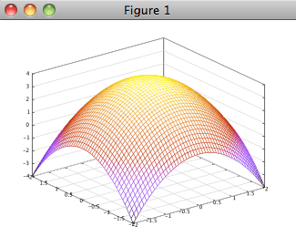
>>> x=linspace(-2,2,50);
>>> y=linspace(-2,2,50);
>>> [xx,yy]=meshgrid(x,y);
>>> mesh(xx,yy,4-(xx.^2+yy.^2))

You can get a contour plot by using the command meshc.

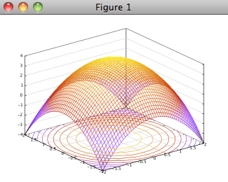
>>> x=linspace(-2,2,50);
>>> y=linspace(-2,2,50);
>>> [xx,yy]=meshgrid(x,y);
>>> meshc(xx,yy,4-(xx.^2+yy.^2))