Curves

Apart from plotting the graph of a function, GeoGebra can also plot a curve that is

• defined by an equation in \(x\) and \(y\),
• the locus of a point satisfying some condition,
• a parametric curve.

Load GeoGebra worksheet

Implicit functions

GeoGebra distinguishes between explicit functions and functions that are defined implicitly by equations in \(x\) and \(y\).

An explicit function is written by using brackets ‐ using \(f(x)\)-notation.

An implicit function can be written as \(y=x^2\). In this case \(y\) can be expressed explicitly in terms of \(x\) and the curve shown, could also be shown as the graph of the function \(f(x) = x^2\). An implicit function however, can also have several \(y\)-values corresponding to a \(x\)-value. An implicit function is hence a more general concept than a function. An equation describes a relation between \(x\) and \(y\), and it is not always the case that \(y\) can be expressed explicitly in terms of \(x\). The equation \(x^2+y^2=1\) defines a curve that is the unit circle. All points \((x, y)\) satisfying the equation lie on the curve. The curve is implicitly defined by the equation.

GeoGebra categorizes a curve defined by an equation as a Line, a Conic, or as an Implicit curve.

GeoGebra can create implicit curves defined by equations, if the equations are written using polynomials in \(x\) and \(y\). If you, for instance, write y = sin(x) GeoGebra will classify this as function, a function that will be given a name by GeoGebra.

Commands that take a function as argument, do not work on conic sections or lines. If a is defined by the equation y=x^2, you cannot use the command TurningPoint on a. In order to use commands for functions, write it as a function, i.e. use \(f(x)\)-notation!

Locus

If you have a point satisfying some condition, then the set of all such points is a locus.

To make a locus in GeoGebra, you need a point \(B\) that depends either on another point \(A\) or a slider. The point \(A\) must lie on a curve or a coordinate axis. Using the tool Locus you can then create the locus by first clicking on \(B\) and then on \(A\) or the slider.

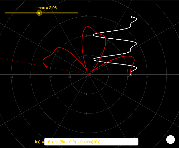
Polar coordinates

In GeoGebra you can use polar coordinates when defining a point. When using polar coordinates, a semicolon is used as delimiter, as in A=(r;α). By letting the angle get its value from a slider \(t\), and by defining a function \(r(x)\), it is possible to draw the curve traced out by a point A=(r(t);t). Use the tool Locus, click on the point and then the slider. Under the preferences for Graphics, under the Grid tab, it is possible to show the grid in polar form.

Polar coordinates can be converted to Cartesian coordinates by letting \(x=r\cos(t)\) and \(y=r\sin(t)\). This can be used for drawing the curves as parametric curves instead of a locus.

Parametric curves

If the \(x\)- and the \(y\)-coordinate both depend on a parameter \(t\), they describe a parametric curve with parameter \(t\). Each point on the curve can be described by the coordinates \((x(t),y(t))\). By letting \(t\) start at a value \(start\) and end at a value \(stop\) you can draw the curve \(k\) by entering:

k = Curve( x(t), y(t), t, start, stop)

in the input bar.

You can always convert a regular function to a parametric function. As an example, the graph of \(f(x)=x^2,-10\leq x \leq 10\) can be drawn as a parametric curve by writing the code:

k = Curve(t, t^2, t, -10, 10)

By letting a slider represent the stop-value, it is possible to visualize how a graph is drawn. Create a slider tmax and define the curve as:

k = Curve(t, t^2, t, -10, tmax)

Transformations and curves

The only transformation you can use on the graph of a regular function is Translate by Vector.

Apart from translating a parametric curve, you can also transform it by using the transformations Reflect about Line and Rotate around Point.

Exercises

Exercise 1

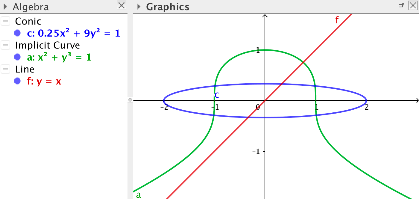
Make conic sections

Create four sliders \(a\), \(b\), \(h\) and \(k\).

In analytic geometry a parabola can be defined by the equation

an ellipse by the equation

and a hyperbola by the equation

Create the three conic section using these equations.

What effect do the values of \(h\) and \(k\) have on the three curves?

What effect do the values of \(a\) and \(b\) have on the ellipse and on the hyperbola?

Exercise 2

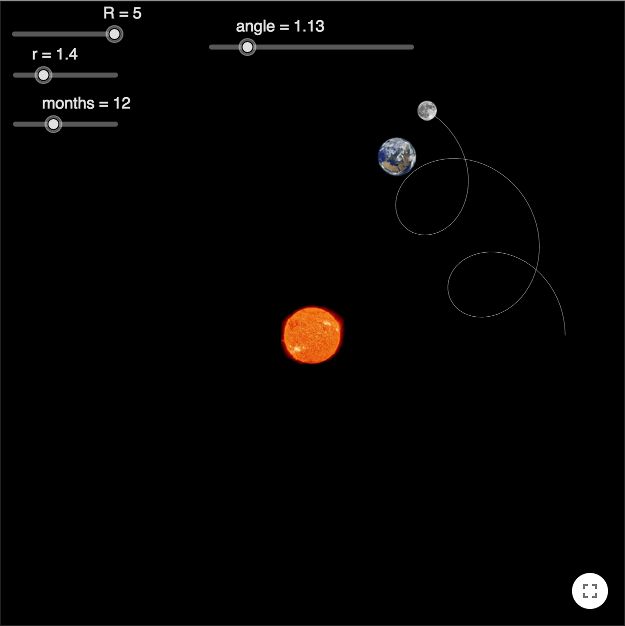
Sun, earth and moon

Create a slider \(R\) representing the radius of the trajectory of the earth moving around the sun.

Create a slider \(r\) representing the radius of the trajectory of the moon moving around the earth.

Create a slider \(m\) taking integer values representing the number of months in a year.

Place a point \(S\) (the sun) at the origin.

Version 1 ‐ using degrees and rotations

Create a slider \(\alpha\) taking angle values representing the angle of the earth.

Place a point \(E\) (the earth) on the positive \(x\)-axis. The distance between \(S\) and \(E\) should be \(R\). Use the tool Rotate around Point to rotate \(E\) around \(S\) the angle \(\alpha\). The rotated point will be called \(E'\). Hide the point \(E\).

Create a point \(M\) (the moon) by writing M = E'+(r, 0). Now \(M\) should be rotated around \(E'\) by an angle depending on the number of months \(m\) and the angle \(\alpha\). Find this angle and create the rotated point \(M'\). Hide \(M\).

Use the tool Locus. First click on \(M'\) and then on the slider \(\alpha\).

Version 2 ‐ using radians and trigonometry

Create a slider \(a\) with values between \(0\) and \(2\pi\) representing the angle of the earth.

Let the point \(E\) represent the earth. Find the \(x\)- and \(y\)-coordinate of \(E\) in terms of appropriate sliders. Enter the expression for the point in the input bar.

Let \(M\) represent the moon. Find the \(x\)- and \(y\)-coordinate of \(M\) in terms of appropriate sliders. Enter the expression for the point in the input bar.

The expressions used for the coordinates of the moon, can also be used to make a parametric curve showing the path of the moon. Create this curve. Let the parameter start with the value \(0\) and end with the value \(a\).

Comment: It is possible to show images instead of points. The images in the worksheet below are from NASA's image gallery.

Load GeoGebra worksheet

Exercise 3

Domain and range for inverse trigonometric functions

If \(f^{-1}\) is the inverse function of a function \(f\), then the graph of \(f^{-1}\) is the reflection of the graph of \(f\) in the line \(y = x\).

In order to reflect a graph, it must be made as a parametric curve.

• Define the function f(x) = sin(x). Hide the graph.

• Place two points \(A\) and \(B\) on the \(x\)-axis. The points represent the end points of the domain of the function.

  You can show the \(x\)- or \(y\)-coordinate of a point as a label. Write %x or %y as Caption in the properties window.

• Create the parametric curve to the function \(f(x)= \sin(x), x(A) \le x \le x(B)\).

• Reflect the curve in \(y=x\). You can either use the tool Reflect about line or use the command Reflect( <Object>, <Line> ).

• Link \(f\) to an input box using the tool Input Box so you easily can redefine the function.

• Drag the points. Study the intervals for which the reflected curve could be the graph of a function. In those cases, what is the domain and what is the range of the inverse function?

Exercise 4

Make a Lissajous curve

A Lissajous curve appears from a periodic motion along the \(x\)-axis and one along the \(y\)-axis.

A Lissajous curve can be described by an equation

An easier equation is used in the worksheet below.

Load GeoGebra worksheet

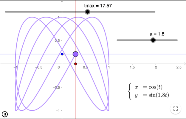
Visualize a Lissajous curve in such a way that the two periodic motions along the coordinate axes are also shown.

You can also make damped Lissajous curves, see Damped Lissajous Curves for more information.