Differential Equations
Using the GeoGebra command solveODE you can illustrate numerical solutions to first and second order ordinary differential
equations.
First order differential equations
When using the command solveODE, \(y\) must be a function of \(x\). Let
then you can used the commands:
solveODE(f)
solveODE(f, <Point on f>)
solveODE(f, <Start x>, <Start y>, <End x>, <Step>)
and:
SlopeField(f)
SlopeField(f, <Number n>)
SlopeField(f, <Number n>, <Length multiplier a>)
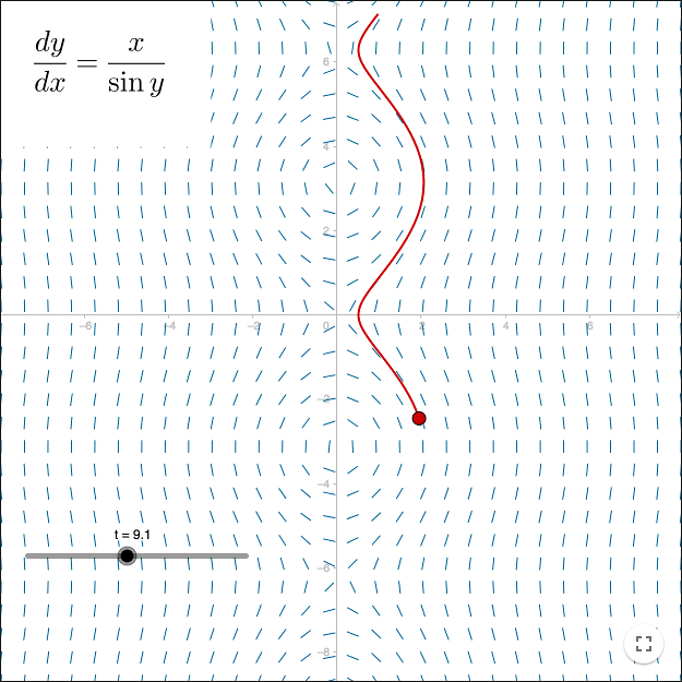
If the solution curve has vertical points and if the equation can be written as
\[\frac{dy}{dx} = \frac{f(x,y)}{g(x,y)}\]it is better to use the command
solveODE(f, g, x(A), y(A), <End t>, <Step> )
where A is a point on the curve. This command is used in the worksheet above.
Second order differential equations
The command
SolveODE[<b(x)>,<c(x)>,<f(x)>,<Start x>,<Start y>,<Start y'>,<End x>,<Step> ]
solves the equation
\[y''+b(x)y'+c(x)y=f(x)\]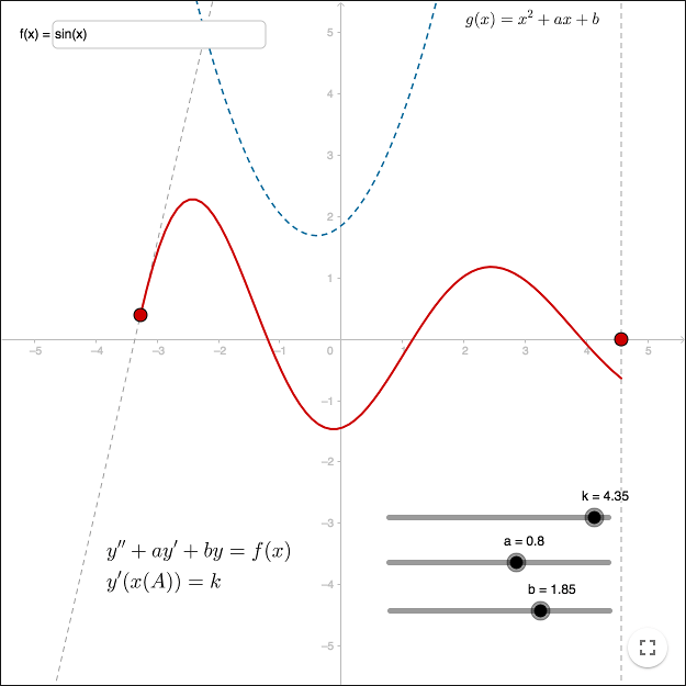
Exercises
Exercise 1
First order ODE
Make the function
\[f(x, y) = y\sin(x) + \frac{y}{x}.\]Link an input box to the function so you easily can redefine it.
Make a point \(A\).
Make a slope field and solve the equation numerically.

by Malin Christersson under a Creative Commons Attribution-Noncommercial-Share Alike 2.5 Sweden License