Linear Functions
Slope


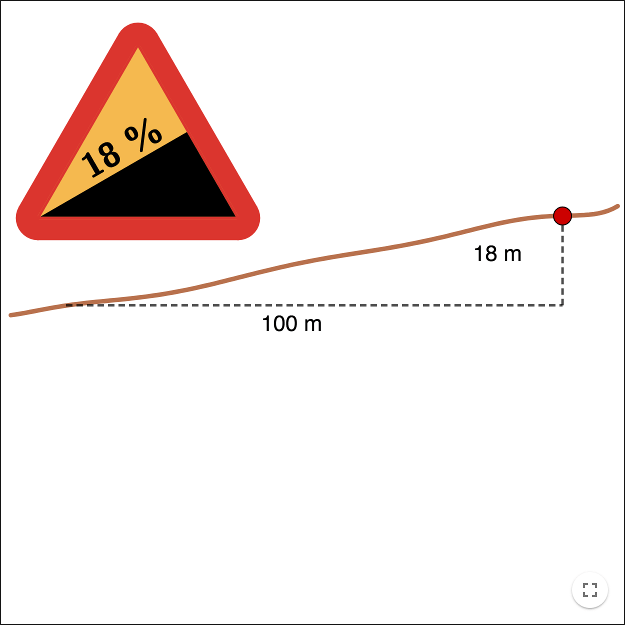
The ten percent slope in the road signs above mean that if you move 100 m along the horizontal direction, then you move at an average 10 m along the vertical direction.
In order to find the percentage slope, you divide the movement along the \(y\)-axis with the movement along the \(x\)-axis, \(\frac{10}{100}=0.1=10\)%.
The road signs above assume that you drive from the left to the right, from the look of the pictures you can deduce whether it is a slope downwards or upwards.
When defining slope in mathematics, the definition is similar to the slopes on the road signs. The slope is defined to be the difference along the \(y\)-axis divided by the difference along the \(x\)-axis. In order to distinguish between a slope downwards and a slope upwards, the difference along the \(y\)-axis is counted as negative if the slope is downwards when going from the left to the right.

Instead of the words "difference along", the symbol \(\Delta \) is used. The difference along the \(y\)-axis is denoted by \(\Delta y\) and the difference along the \(x\)-axis by \(\Delta x\).
If \(m\) denotes the slope, then \(m\) is given by
\[m=\frac{\Delta y}{\Delta x}\]Measuring slope with GeoGebra
If you have a line in GeoGebra, you can measure the slope of the line by using the tool ![]() Slope.
Slope.
GeoGebra shows the slope in such a way that \(\Delta x\) always is equal to one.

The GeoGebra-way of defining slope could be seen as an alternative definition:
If the change along the \(x\)-axes (moving from left to right) is 1,
then the change along the \(y\)-axes is the slope.
The equation of a line
The equation of a line can be written in slope-intercept form as
\[y = mx + c,\]where \(m\) is the slope and \(c\) is the \(y\)-intercept. Vertical lines cannot be written this way since the slope isn't defined for vertical lines. Instead a vertical line is written as
\[x = c,\]for some constant \(c\).
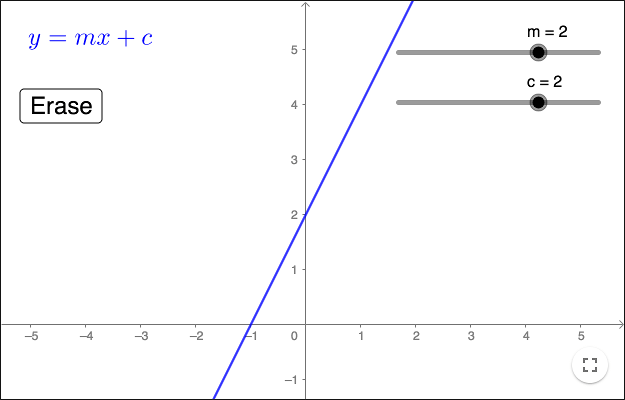
Erase and change \(c\) to see many lines with the same slope.
Slope-point form
If you know that a point \((h, k)\) lies on a line, and you know that the slope of the line is \(m\), then you can write the equation of the line as
\[y = m(x-h)+k.\]General form
When using general form to write the equation of a line, you write the equation as
\[ax+by=c.\]The major difference between this form and slope-intercept form is that we now have a coefficient \(b\) in front of \(y\). When \(b=0\) the line is a vertical line.
Linear functions
A linear function is a function whose graph is a line. A linear function can be written as
\[y = mx + c,\]or as
\[f(x) = mx +c.\]Note that if you enter \(y = mx + c\) in GeoGebra, where \(m\) and \(c\) either are represented by sliders or written by using numbers, then the line is given a function name \(f\).
Linear and exponential growth
In you want to model a situation where something that grows with the same amount for each time step, you can use a linear function. There is a big difference between this so-called linear growth and if you have something that grows by a percentage change, in which case you have an exponential growth.
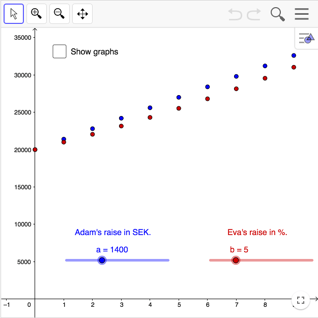
Adams has a linear raise and Eve an exponential.
"Altogether, Adam lived 930 years, and then he died."
Show the graphs. Zoom out to check out Eve's salary 930 years later!
Exercises
Exercise 1
Gradients of Perpendicular Lines
Draw a line through points \(A\) and \(B\).
Draw a line perpendicular to the first line through the point \(A\).
Use the tool
 Slope
on both lines.
Slope
on both lines.Rename the gradients to \(m_1\) and \(m_2\).
Make a new variable \(product\) by writing:
product = m_1*m_2
Move the points! Make a conjecture about the product! Prove your conjecture!
Hint: Look at the slopes shown by GeoGebra and try to use similar triangles.
Exercise 2
Linear and percentage increase
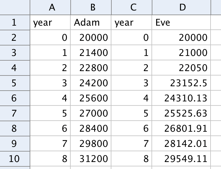
Adam and Eve both have a monthly salary of 20,000 SEK. Adam negotiates to get a pay raise of 1400 SEK per year in monthly salary. Eve negotiates to get 5% increased monthly salary per year.
2.a - Show the pay raises by using fix numbers
Use two columns to represent the years, column A for Adam and column C for Eve. Make them by using relative copies.
Enter 20000 into B2 and D2. Write a spreadsheet-formula for Adam's pay raise by 1400 SEK in B3. Make relative copies along column B. Find the factor of change representing a percentage increase by 5%, and use this factor to write a spreadsheet-formula for Eve's pay raise in cell D3. Make relative copies along column D. The cells should show the salaries for the next 20 years.
Make two lists of points, one for Adam and one for Eve. Make sure that the points are shown in the drawing pad.
2.b - From fix numbers to variables
Store the value 1400 in a variable \(a\), and the factor for Eve in a variable \(e\) (enter the variables in the input bar). Change the spreadsheet-formulas in cells B3 and D3 so the variables are used instead of the fix numbers. Make new relative copies along columns B and D.
Make two new lists of points. Change the values of the variables by right-clicking on them and enter the properties window. Change the value for Adam to 2000 SEK and make Eves yearly increase 8%. When you change the value of a variable, all cells that depend on that value are changed and also all points.
2.c - From variables to sliders
The two variables can be seen in the algebra view. Click on the small circles to make them filled. By doing so, two so called sliders are created. Using a slider, you can change the value of a variable.
Open the properties window for each of the sliders. See to it that Adam's pay raise can be varied between 0 and 10000 SEK, and that Eve's can vary between 0 and 50%.
Exercise 3
Annuity loan using variables
When borrowing money using an annuity loan, you repay the same amount of money each year.
When doing calculations using an annuity loan, you use so called geometric series. You can, however, show the debt over time by using a spreadsheet without using geometric series.
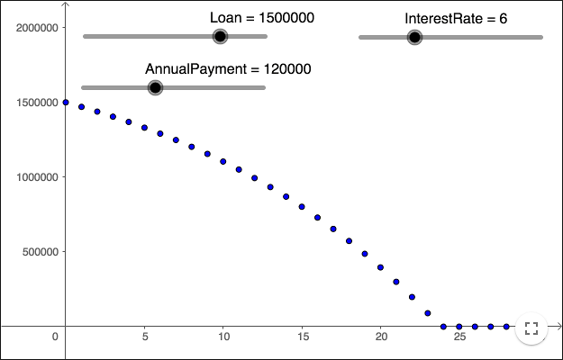
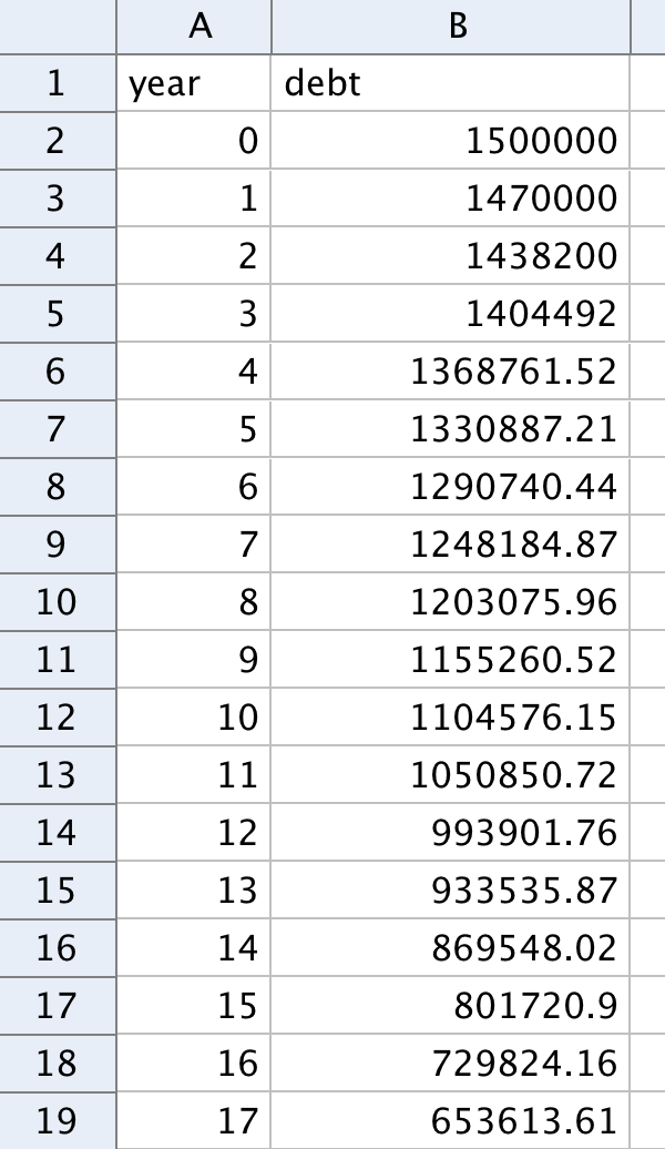
To model an annuity loan, you need three variables; one to represent the loan, one to represent the annual interest rate, and one to represent the annual payment. Make three variables and let the loan be 1 500 000 SEK, the interest rate 6%, and the annual payment 120 000 SEK.
Let column A represent the years and column B the remaining debt. See the picture to the right.
Enter the variable for the loan in cell B2.
Cell B3 should contain the spreadsheet-formula for the debt after one year, after first increasing the debt by using the factor for percentage increase and then decreasing the debt by one annual payment. Make relative copies to show the remaining debt for 30 years.
Visualize the remaining debt in the graphics view as points.
Change all variables to sliders, so you can change the values.
If you want the remaining loan never to be negative, as in the worksheet above, you can take the maximum of your formula and zero.
Max(<your formula>, 0)
Let the annual interest rate be 8% and the let the loan be 1 500 000 SEK. Try out various annual payments.
Answer following question:
How large must the annual payment be in order to guarantee that the loan has been repaid in at most 30 years if the loan is 1 500 000 SEK and the annual interest rate is 8%?
reference:
the pictures of the road signs are from: http://commons.wikimedia.org/wiki/Category:Slope_signs
by Malin Christersson under a Creative Commons Attribution-Noncommercial-Share Alike 2.5 Sweden License