De Casteljau's Algorithm and Bézier Curves
| ←Damped Lissajous Curves | How to Make a Cubic Bézier Spline→ |
|---|
The geometric construction
Bézier curves are used to draw smooth curves along points on a path. A Bézier curve goes through points called anchor points and the shape between the anchor points is defined by so called control points.
JavaScript is needed!
Move the red points!
Movement between two points using vectors
A point \(Q\) that moves from \(P_1\) to \(P_2\) over the time \(0\le t \le 1\) can be described using position vectors. Let \(O\) be some fixed point, then the position vector \(\vec{OQ}\) points at \(Q\). Let \(\vec{P_1P_2}\) be the vector between \(P_1\) and \(P_2\), then \(\vec{OQ}\) is described by
\[ \vec{OQ} = \vec{OP_1}+t\vec{P_1P_2}, t\in[0,1]. \]To find the coordinates of \(\vec{P_1P_2}\), position vectors are used,
\[ \vec{P_1P_2} = \vec{OP_2}-\vec{OP_1}. \]We get
\[ \vec{OQ} = \vec{OP_1}+t\vec{P_1P_2} = \vec{OP_1}+t(\vec{OP_2}-\vec{OP_1}) =(1-t)\vec{OP_1}+t\vec{OP_2}. \]The position vector of a point has the same coordinates as the point. For that reason you don't have to distinguish between points and vectors when doing computer graphics. The point \(Q\) can be written as
\[ Q = (1-t)P_1+tP_2, t\in[0,1]. \]Parametric equation of a Bézier curve
Linear Bézier curves: Two points \(P_0\) and \(P_1\) are needed. Both are anchor points. As \(Q_0\) moves along the line between \(P_0\) and \(P_1\) it traces out a linear Bézier curve. Let \(t\) be a parameter, then the linear Bézier curve can be written as a parametric curve
\[ Q_0=(1-t)P_0+tP1, t\in [0,1]. \]Quadratic Bézier curves: Three points \(P_0, P_1, P_2\) are needed. \(P_0\) and \(P_2\) are anchor points. \(P_1\) is a control point. The \(Q\)-points move along lines between the \(P\)-points. As \(R_0\) moves along a line between \(Q_0\) and \(Q_1\), it traces out a quadratic Bézier curve. The three movements along lines are described by
\[ \begin{align*} Q_0 &=(1-t)P_0+tP1, t\in [0,1] \\ Q_1 &=(1-t)P_1+tP_2, t\in [0,1] \\ R_0 &=(1-t)Q_0+tQ_1, t\in [0,1] \end{align*} \]Just using the \(P\)-points to describe \(R_0\) we get that
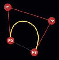
\[ R_0 = (1-t)^2P_0+2(1-t)tP_1+t^2P_2, t\in [0,1]. \]Cubic Bézier curves: Four points \(P_0, P_1, P_2, P_3\) are needed. \(P_0\) and \(P_3\) are anchor points, the others are control points. Just using the \(P\)-points to describe \(S_0\) we get that
\[ S_0 = (1-t)^3P_0+3(1-t)^2tP_1+3(1-t)t^2P_2+t^3P_3, t\in [0,1]. \]Quartic Bézier curves: Five points \(P_0, P_1, P_2, P_3, P_4\) are needed. \(P_0\) and \(P_4\) are anchor points, the others are control points. Just using the \(P\)-points to describe \(T_0\) we get that
\[ T_0 = (1-t)^4P_0+4(1-t)^3tP_1+6(1-t)^2t^2P_2+4(1-t)t^3P_3+t^4P_4, t\in [0,1]. \]The divide-and-conquer-algorithm
The equations of the parametric curves can be used to draw a Bézier curve. They can also be used to explain how to draw the Bézier curve using a divide-and-conquer-algorithm. The geometric construction can be used to split a curve in two halves, and then draw the curve using the algorithm:
draw a line segment between the starting
point and endpoint;
otherwise
split the curve and draw each of the halves
recursively.
As we zoom in on the curve, it will get flatter and flatter. Therefore the recursion will end! We only need to know how to split a curve, and how to define "flat enough".
How to split a Bézier curve
JavaScript is needed!
If the curve is split at \(t=0.5\), we get two curves represented by the movement of points along the first half of their respective line segments, and by the movement along the second half.
In the cubic example above, the original curve is defined by the anchor points \(P_0\) and \(P_3\), and the control points \(P_1\) and \(P_2\). When \(t=0.5\), the \(Q\)-points are midpoints between \(P\)-points, and the \(R\)-points are midpoints between \(Q\)-points.
After the split, one curve is defined by anchor points \(P_0, S_0\) and control points \(Q_0, R_0\); the other curve is defined by anchor points \(S_0, P_3\) and control points \(R_1, Q_2\). All the defining points are midpoints between other points.
Defining "flatness"
One way to define flatness is to consider how close the control points are to the anchor points. It is easy to see that
\[ \frac{|P_0P_1|+|P_1P_2|+|P_2P_3|}{|P_0P_3|}\geq 1. \]In order to define "flat enough", pick some "flatness factor" and check if
\[ |P_0P_1|+|P_1P_2|+|P_2P_3| < \text{"flatness factor"} \cdot |P_0P_3| \]When using de Casteljau's divide-and-conquer-algorithm, the length of each line segment depends on the flatness of the curve.
JavaScript is needed!
Animated gifs
Animated split curve on tumblr.
